1. Fourier Analysis
Fourier Analysis is a very powerful tool that comes into play when we discuss periodic signals. Colloquially, a periodic signal repeats.
3.1. Introduction
Mathematically a signal \(x(t)\) is periodic if there exists a positive constant \(T\) such that: \(x(t) = x(t + T)\) for all values of \(t\). The smallest value of \(T\) for which this is true is called the fundamental period and is denoted \(T_o\). The corresponding fundamental frequency is \(f_o = \frac{1}{T_o}\). If \(T_o\) is in seconds, then \(f_o\) is in Hertz (Hz). The fundamental angular frequency is \(\omega_o = 2\pi f_o\) and is measured in rad/sec.
3.2. Fourier Series
A Fourier series is an expansion of a periodic function f(x) in terms of an infinite sum of sines and cosines. The computation and study of Fourier series is known as harmonic analysis and is extremely useful as a way to break up an arbitrary periodic function into a set of simple terms that can be plugged in, solved individually, and then recombined to obtain the solution to the original problem or an approximation to it to whatever accuracy is desired or practical. 1
Mathematically in a simple sense an arbitrary function \(f(t)\) can be decomposed as:
\[f(x) = a_0 + \sum_{n=1}^{\infty} a_n cos(nx) + b_n sin(nx)\]We shall explore this concept by making two waveforms using sinosoids:
3.2.1. A Sqaure Wave
From Lab 1, we have the function generator. We use that to make a square wave of amplitude = 1.
Mathematically it can be written as:
\[f(x) = \begin{cases} 0 & \text{if } -\pi \leq x \lt 0 \\ 1 & \text{if } 0 \leq x \lt \pi \end{cases}\ and\ f(x+2\pi)=f(x)\]Which has a period of \(2\pi\). For an arbitrary period P:
\[f(x) = \begin{cases} 0 & \text{if } -P/2 \leq x \lt 0 \\ 1 & \text{if } 0 \leq x \lt P/2 \end{cases}\ and\ f(x+P)=f(x)\]The corresponding Fourier series of the square wave with period \(2\pi\)
\[f(x) = \frac{1}{2} + \sum_{n=1}^{\infty} \frac{2}{(2k-1)\pi} sin[(2k-1)x] \\ \ \ \ = \frac{1}{2} + \frac{2}{\pi}sin(x) + \frac{2}{3\pi}sin(3x) + \frac{2}{5\pi}sin(5x) + \frac{2}{7\pi}sin(7x) + ... + + \frac{2}{n\pi}sin(nx)\ (\ n\ is\ odd)\]and for arbirary period P:
\[f(x) = \frac{1}{2} + \sum_{n=1}^{\infty} \frac{2}{(2k-1)\pi} sin[\frac{2\pi}{P}(2k-1)x] \\ \ \ \ = \frac{1}{2} + \frac{2}{\pi}sin(\frac{2\pi}{P}x) + \frac{2}{3\pi}sin(\frac{2\pi}{P}3x) + \frac{2}{5\pi}sin(\frac{2\pi}{P}5x) + \frac{2}{7\pi}sin(\frac{2\pi}{P}7x) + ... + + \frac{2}{n\pi}sin(\frac{2\pi}{P}nx)\ (\ n\ is\ odd)\]Use more and more sources to add additional sinusoids and see what waveform you get after each added term. How many terms until you’re square wave looks good? 5? 10?
It should look similar to this:
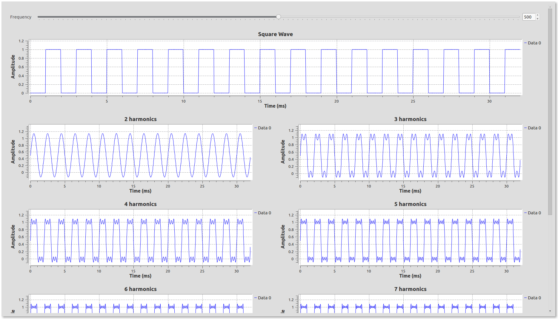
This type of analysis is important for digital design in the sense that most digital signals are square waves, representing either a 1 or a zero. So if your signal is at 10MHz, how fast should the electronics and design work?
3.2.2. A Triangle Wave
The triangular wave is defined as: \(f(x)=|x|\ for\ -1\lt x \leq 1\ and\ f(x+2)=f(x)\ for\ all\ x\)
Its corresponding fourier series is:
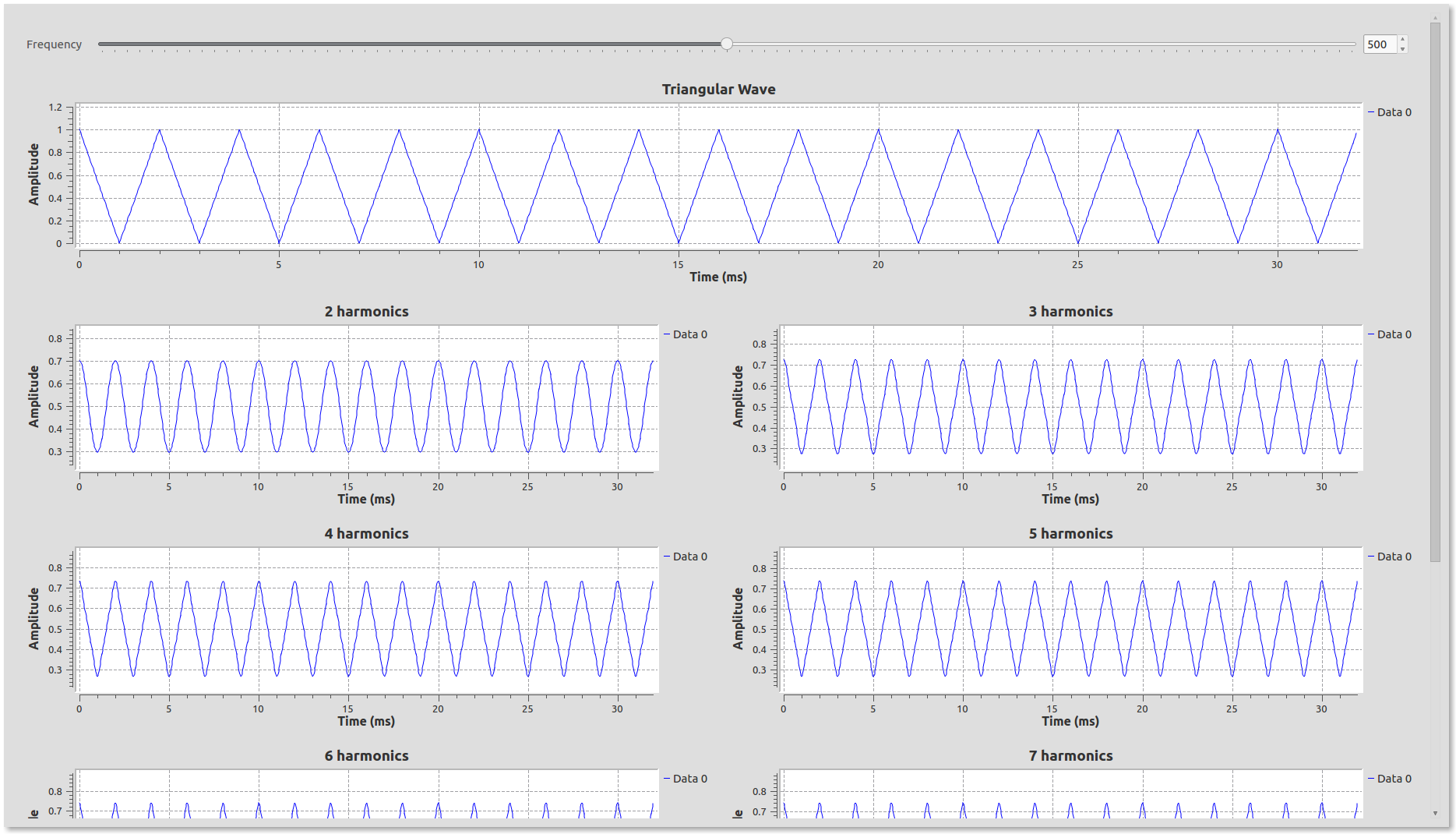
\[f(x) = \frac{1}{2} - \sum_{n=1}^{\infty} \frac{4}{(2k-1)^2\pi^2} cos[(2k-1)\pi x] \\ = \frac{1}{2} - \frac{4}{\pi^2}cos(\pi x) - \frac{4}{9\pi^2}cos(3 \pi x) - \frac{4}{25\pi^2}cos(5\pi x) - ...\]Make a flowgraph out of the expanded terms above and check the output after each operation. Do you need more or fewer components to begin looking like a triangle wave as compared to a square wave? Why do you think that is?
It should give an output like this:
3.2.3. A Sawtooth wave.
Now mathematically define a sawtooth wave and find it’s Fourier series expansion. Then create its flow-graph, again with more and more Fourier components. Again, do you need more/less Fourier components as compared to a square or triangle wave?
3.3. Fourier Series and Fourier Transforms
We segue into the concept of Fourier transforms directly by seeing how they relate to fourier series. First some mathematics to associate familiarity, the Fourier transform of \(x(t)\) is given by:
\[X(\omega) = \int_{-\infty}^{+\infty} x(t) cos(\omega t)dt -i \int_{-\infty}^{+\infty} x(t) sin(\omega t) = \int_{-\infty}^{+\infty}x(t)e^{-i\omega t}dt\]When x(t) is periodic and has a Fourier series expansion, this integral is pulling out those sines and cosines in the expansion.
In more detail: For the complex representation of a Fourier series of a periodic function \(x(t)\) :
\[x(t) = \sum_{-\infty}^{\infty} c_n e^{jn\omega t}\]The co-effecients, \(c_n\) of \(x(t)\) (which has the period \(T\) is given by the relation:
\[c_n = \frac{1}{T} X(n\omega_o)\]where \(X(\omega)\) is the Fourier transform and \(\omega_o = \frac{2\pi}{T}\)
In summary, the Fourier series of a signal is a sum of sines and cosines. And, the Fourier transform decomposes the signal into it’s its frequency components with their relative strength. This can be visually seen in a neat animation as shown below ( credit: wikipedia ) and in the next section
3.3.1. Fourier Transform
Use the Square Wave and the Triangle Wave flowgraphs from the previous exercise.
First use a signal source block to make a square wave and feed the signal into a QT frequency sink
The Frequency Sink takes the Fourier Transform of the incoming signal and plots the output of the fourier transform
Place another QT Frequency Sink and change the number of inputs to the number of Fourier series sinusoids you have in your flowgraph and feed all the sinusoids (vis-a-vis the individual Fourier series terms) into the frequency sink
The output looks like this:
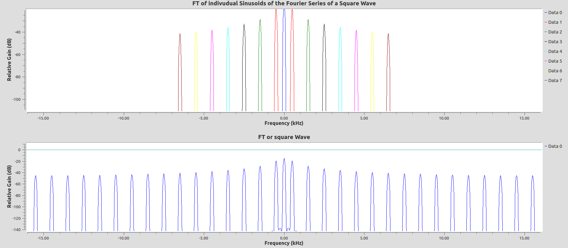
The colored peaks are the Fourier transforms of the individual sinusoids. Do they align with the Fourier Transform of the pure square wave? If you add more terms of the Fourier series to the sink, how do they compare?
Repeat this exercise for the triangle wave.
We’ve been taking Fourier transform of the signal every time we see a plot with frequency in the time axes.
We shall visit Fourier transforms in detail again that in Lab 5.
3.3.2. Example
We can also think of this to use gnuradio-companion to graphically get the Fourier components of a signal using a Fourier transform. Create a flow-graph with a signal source->FFT(Fourier transform)-> complex to real/imag -> vector sinks. The output of the real-part contains the cosine components of the transform. The imaginary part contains the sine components of the Fourier expansion.
It is also helpful to plot the time series to see what your input is and the frequency sink to make it easier to just read off the frequency of the components.
An example flowgraph looks like:
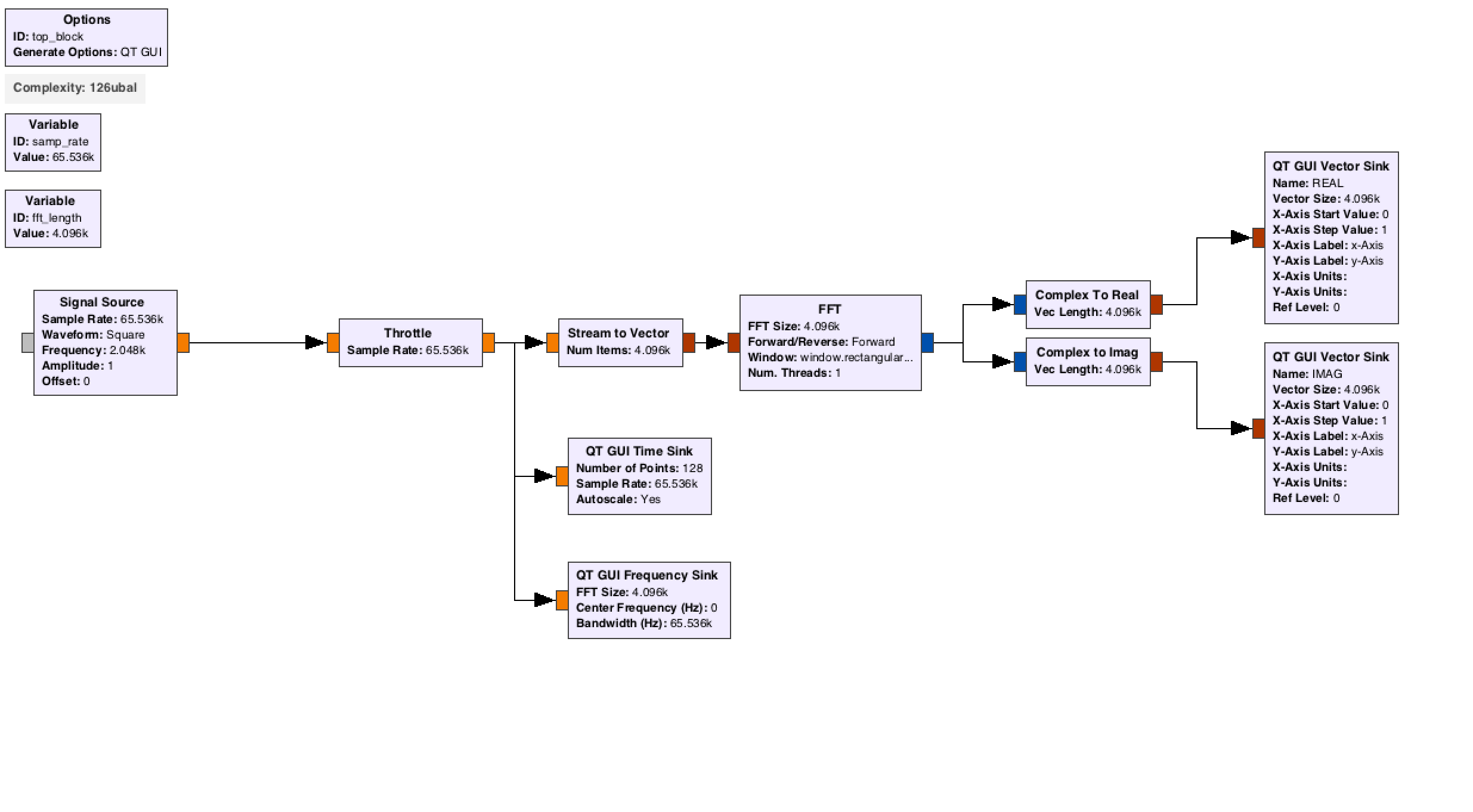
The FFT block is a special block which does the Fourier transform really fast. Play around with the FFT block and your general waveform generator from Lab 1 to take their Fourier transform. Use this to read off the Fourier series coefficients. This can still be used with a periodic signal with much less obvious structure.
3.4. Fourier Transform Pairs
Let us revisit Fourier transform by exploring the concept through their various properties. Refer to this Table of Fourier Transform Pairs and Properties and implement in gnuradio the following :
- Fourier Transform a Sinusoid and
- Fourier transform of the sinusoid delayed by one sample
- The output of the Fourier transform of a constant source of the value 1 is a dirac delta function. Find the FT of the dirac delta function and the dirac delta function time delayed.
- Fourier transform of \(e^{j\omega_o t}\)
- Demonstrate the convolution property (use square wave) Hint: Inverse Fourier transform can be implemented by choosing
reversein theForward/ReverseOption. Hint: The output should be a triangle wave - Fourier transform a square pulse of different widths (i.e. tau refer lab 1.3.1)
Try to implement other properties from the link of fourier transform pairs and properties as well.
NOTE: Use the FFT Block for the above exercises. Use complex sources. The FFT block takes an input vector and outputs a complex vector. Use to appropriate stream to vector and complex to real/imaginary convertor blocks where necessary
The power of the FFT output is given by multiplying the complex output of the FFT by its complex conjugate
Use vector sinks for signals that ‘vectors’ i.e. data comes out in chunks of a particular matrix size(vector length)
↑ Go to the Top of the Page ……Next Lab
-
http://mathworld.wolfram.com/FourierSeries.html ↩