
4. Digital Filters
A filter changes the nature of the signal. A digital filter does so by manipulating a discretized signal.
- 4. Digital Filters
4.1. Introduction
The previous lab showed how Fourier transforms connect a signal’s time-domain and frequency-domain representations. Information in a signal can be distinctly displayed as a function of the three parameters: time, frequency and phase. Different filters are designed to manipulate the said information in the signal with respect the different parameters.
Use for example the signal x as a function of time: \(x(t) = A cos(\omega t + \phi)\)
A filter can change the signal’s amplitude: \(y(t) = B(\omega) x(t)\). The output will have a different amplitude compared to the input, depending on the frequency.
4.1.1. Filter Terminology
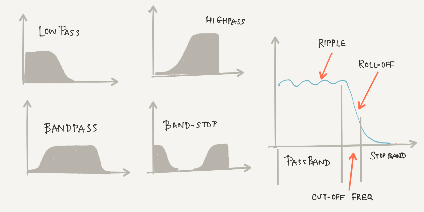
- Cut-off Frequency: The frequency around which the signal either passes or stops
- Low Pass: A filter which allows only frequencies below the cutoff frequency to pass
- High Pass: A filter which allows only frequencies above the cutoff frequency to pass
- Band Pass: A filter which allows only frequencies between a range of frequencies to pass
- Band Stop: A filter which allows only frequencies no within a range of frequencies to pass
- Pass-Band: The range of frequencies through which the signal passes
- Stop Band: The range of frequencies through which no signal passes ideally.
- Ripple: Oscillations from the expected straight line.
- Roll-off: The region between the end of the pass-band and a stop-band.
- Finite Impulse Response (FIR) Filter: Its impulse response reaches zero after a finite time. Feedback is absent or carefully accounted for.
- Infinite Impulse Response (IIR) Filter: A filter with feedback.
4.2. Moving Average Filter
A moving average filter does exactly what its name suggests. It is a very commonly used filter and very simple in its implementation. It performs optimally in the time domain particularly functioning to reduce random noise. It is mathematically represented as:
\[x_{n-point-average} = \frac{x[M]+x[M-1]+ . . . + x[M-(n-1)]}{n} \\ M\ is\ the\ M^{th}\ index\]NOTE: A moving average filter is a simple finite impulse response(FIR) filter. Specifically it is a low-pass filter. You can also think of this as a convolution.
4.2.1. Exercise 1: Noise Reduction
Use a sine wave from the signal source and add noise to it (Discussed in Lab 1). Pass this to a 8-tap moving average filter. The flowgraph should resemble this diagram:
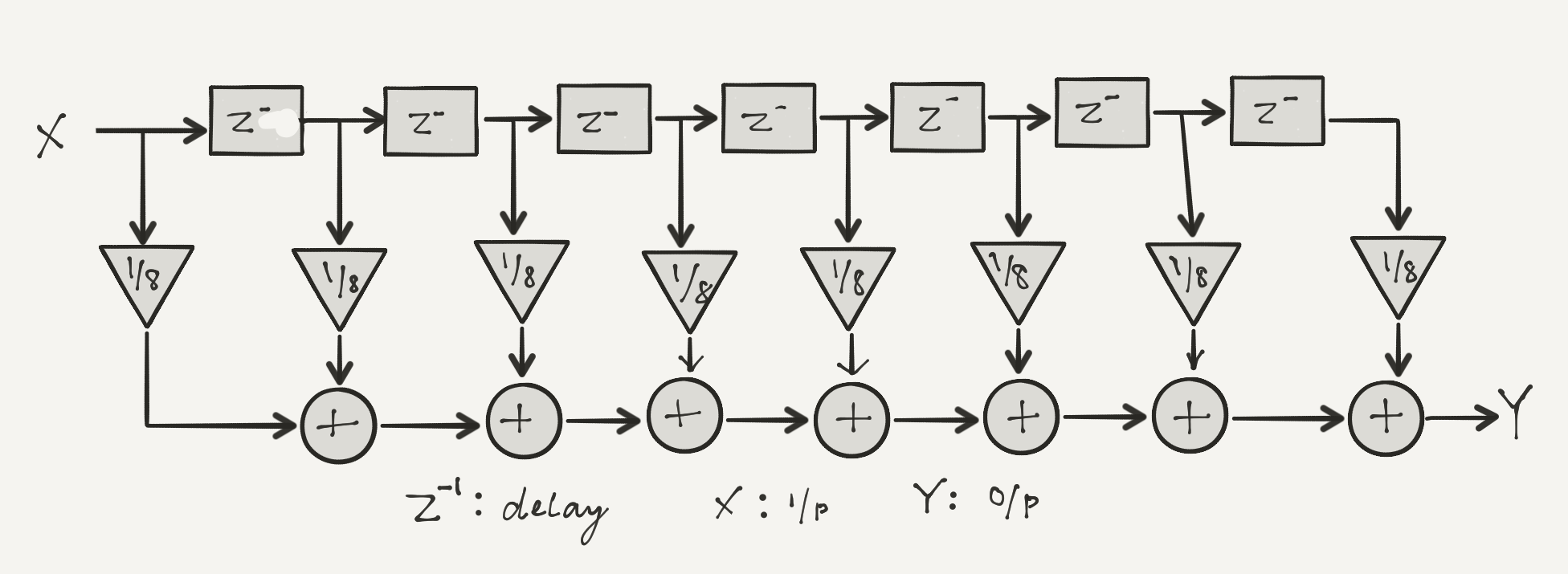
Observe the signal before and after the filtering. Cascade multiple 8 point average filters (i.e. connect end to start). Save the filter as a ‘hier block’. Give it two ‘pad sources’ and two ‘pad sinks’ (why two?). Once the block is compiled, reload the blocks (refresh button in gnuradio-companion). There should now be a “GRC Hier Blocks” section with your block named. How does the signal change adding more and more averaging?
*Note: There are two options for ‘heir’ block with or without ‘QT GUI’ appending heir. Choose the one without the ‘QT GUI. Male sure you have to disabled blocks in your flowgraph *
4.3. FIR: Finite Impulse Response Filters
“A finite impulse response (FIR) filter is a filter whose impulse response (or response to any finite length input) is of finite duration, because it settles to zero in finite time. This is in contrast to infinite impulse response (IIR) filters, which may have internal feedback and may continue to respond indefinitely (usually decaying).”1
The FIR flow diagram is below. \(x[n]\ and\ y[n]\) are input and output, respectively. \(z^{-1}\) is the unit delay. \(b_n\) are filter coefficients.

FIR filters are mathematically fast and relatively easier to design and implement digitally.
We shall design FIR filters using the graphical tool that ships with GNU Radio. Install the additional dependency in a terminal: sudo apt install python-qwt5-qt4. After installation, move the mouse to the window’s top. In the taskbar, click tools, then filter design tool
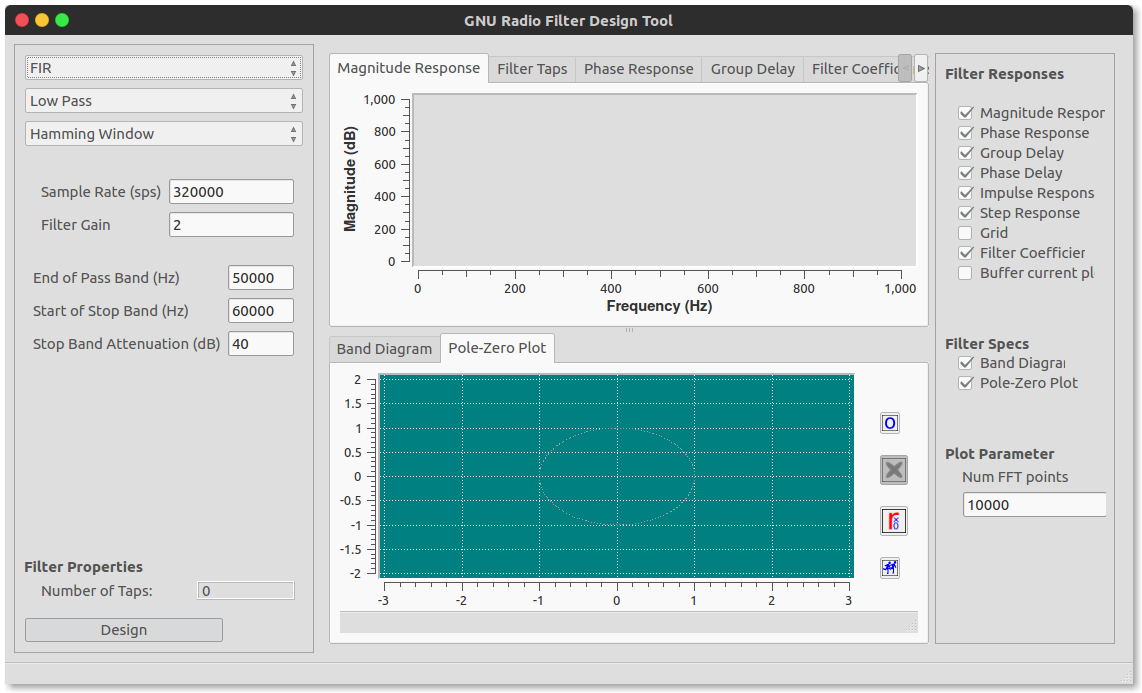
We shall design all our filters by graphically using this tool. Theoretically, there are several methods employed to design a filter. The most common used method is by designing a window function. First, design an ideal filter that may have an infinite impulse response. Multiply that response by a finite window to truncate it. The result is a finite impulse response filter whose frequency response is modified from that of the IIR filter. Multiplying by a window in time convolves the frequency response with the window’s Fourier transform. 1
For us, this GUI does everything behind the scenes. Inspect each filter’s response in the design window. Copy the required taps, or filter coefficients, into the FIR block.
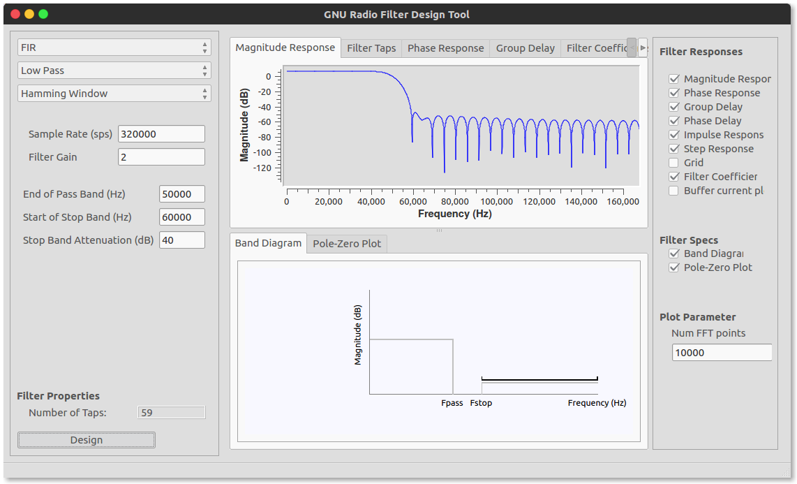
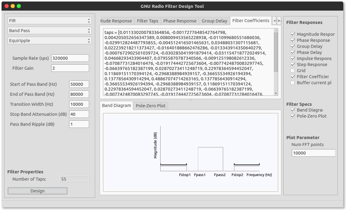
GNU Radio has two kinds of FIR filter blocks. Decimating FIR filters reduce the sample count by division. Interpolating FIR filters increase it by multiplication. Copy the designed Filter Taps into the Taps field in the filter block’s properties.
4.3.1. Exercise 2: Extracting Fundamental Frequencies from a Guitar/Piano Chord (C Major)
A chord is the sound produced by playing three or more notes together. We can use fourier transform to extract the frequencies that make up those chords. Start with an audio source. Convert its float output to complex, then connect it to a Frequency Sink

Once ready, let’s play the C-Major chord. It is the C (= 261.63Hz) , E (= 329.63Hz) and G (= 392Hz). Notice that the frequency spectrum shows more than just the three fundamental frequencies. They show the harmonics of the three frequencies mentioned above! The fundamental and its harmonics combine to form the musical note’s waveform, as described by Fourier series. Different instruments produce different harmonic amplitudes for the same note. These waveform differences contribute to each instrument’s “timbre”.
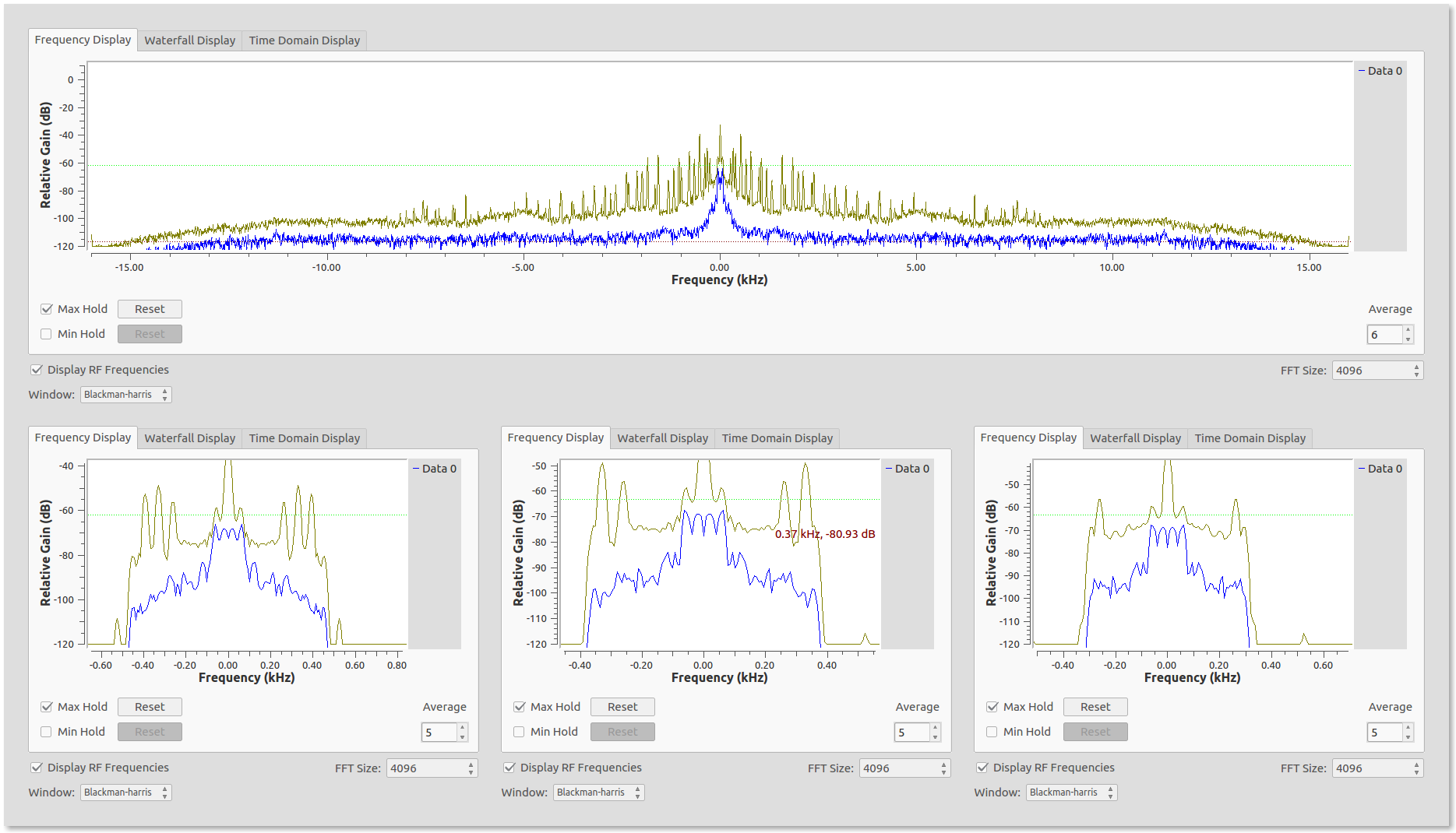
Now let us extract just the fundamental frequencies by implementing low pass filters to have:
- C-E-G Fundamental Frequency ( use cut-off frequency 456 Hz)
- C-E Fundamental Frequency ( use cut-off frequency 361 Hz)
- C Fundamental Frequency ( use cut-off frequency 296 Hz)
The outputs of the filters in the frequency sink should look like this by zooming in:
You may want to save the filtered audio to disk. Look for the the appropriate “sink” block to do so! You can try this with any other chord. Change the filters accordingly. Click here for the frequency of every key on the piano.
Fun Fact: Using Fourier transforms and some cool filtering you can transcribe any chords in any any music piece. For example, deciphering the “mystery” opening chord of the Beatles’ Hard Day’s Night
4.3.2. Exercise 3: Digital Audio Equalizer
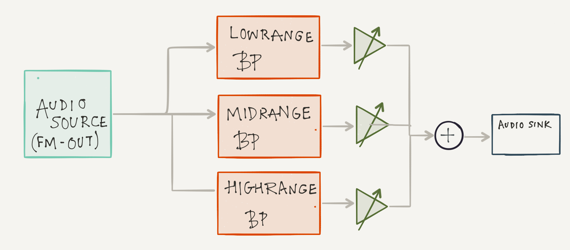
Let us try and construct a simple digital equalizer. This example uses a three-band equalizer. Three band-pass filters define its frequency bands:
- Low range: 20Hz – 250Hz
- Mid-range: 250Hz – 4kHz
- High-range: 4kHz – 20kHz
Attach this to FM Radio flow-graph before the audio sink
The GNU Radio flow-graph will follow this diagram:
You can of course have more than three frequency channels, you can google commonly used frequency divisions in commercial equalizers.
NOTE: “Ancient” stereos/cassette players and old audio workstations in music studios have analog equalizers designed using analog filters. Inspect the equalizer output’s frequency sink to see how well the filters work. Digital filters can be very very precisely designed. The roll-off(or transition width) can be as narrow as you want!
4.3.3. Exercise 4: Guitar Tuner
Let us be more ambitious and design a Digital Guitar Tuner in GNU Radio. Like the equalizer, this uses a series of band-pass filters. Each is centered on a string’s fundamental frequency. The Fundamental frequencies of the open guitar string in a standard tuning:
| String | Frequency |
|---|---|
| 1 (E) | 329.63 Hz |
| 2 (B) | 246.94 Hz |
| 3 (G) | 196.00 Hz |
| 4 (D) | 146.83 Hz |
| 5 (A) | 110.00 Hz |
| 6 (E) | 82.41 Hz |
The flow-graph should resemble this diagram:
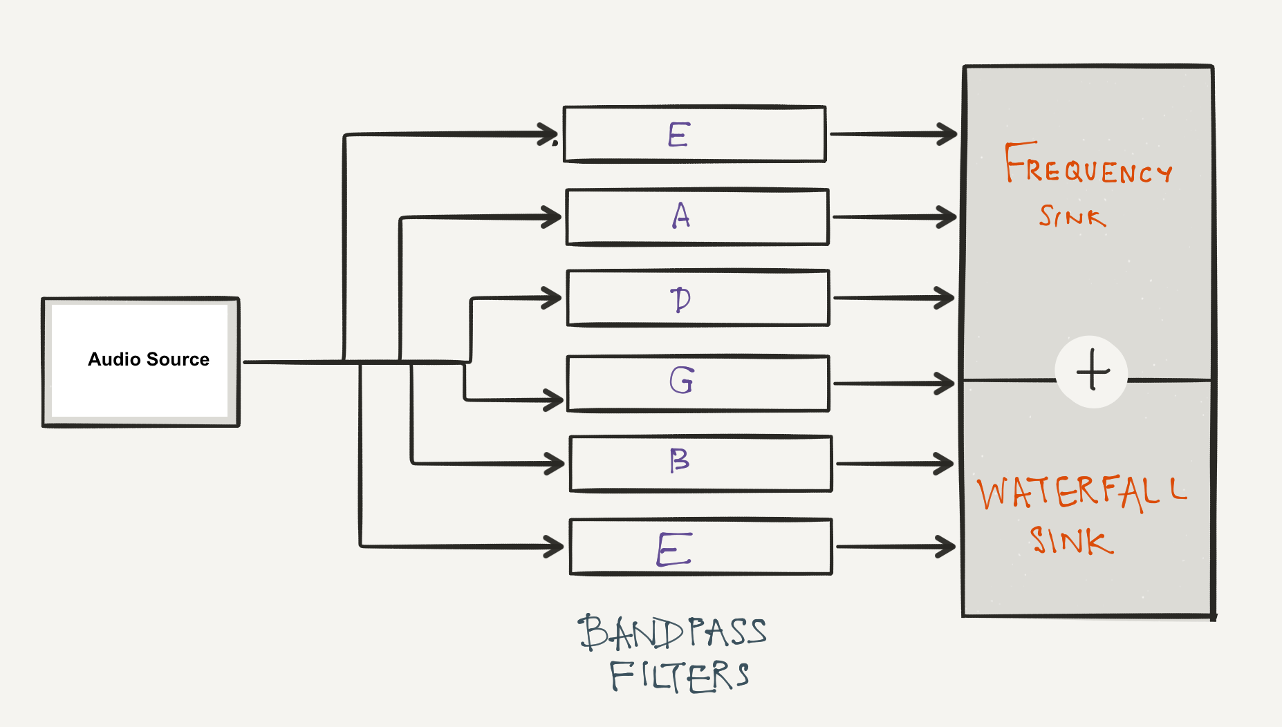
Choose an appropriate bandwidth. Add frequency and waterfall sinks for each string. What type of window will you use?
4.4. IIR: Infinite Impulse Response Filters
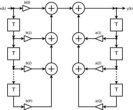
The IIR flow diagram is below. \(x[n]\ and\ y[n]\) are input and output, respectively. \(z^{-1}\) is the unit delay. \(b_n\) are feed-forward coefficients, while \(a_n\) are feedback coefficients.
4.4.1. Classic Analog Filters
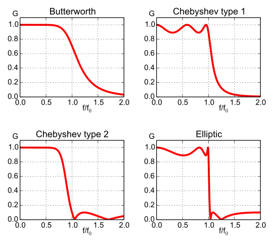
Analog filters use components such as inductors, resistors, capacitors, transistors, and op-amps. Mathematical approximations let us implement these filters digitally. There are 4 types each excelling in one parameter while under-performing in another:
-
Butterworth: Flattest pass-band but a poor roll-off rate.
-
Chebyshev: Some pass-band ripple but a better (steeper) roll-off rate. Chebyshev filters where the ripple is only allowed in the pass-band are called type 1 filters. Chebyshev filters that have ripple only in the stop-band are called type 2 filters , but are are seldom used. Chebyshev filters have a poor phase response.
-
Elliptic: Some pass- and stop-band ripple but with the steepest roll-off rate.
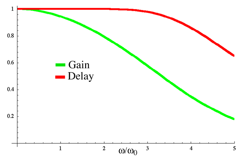
- Bessel: Worst roll-off rate of all four filters but the best phase response.
IIR or Infinite response filters are the closest digital implementations of these filters.
4.4.2. IIR Filter Design
Now create an IIR filter to again pull out the fundamental frequency of the C-chord. Do this again using the ‘Filter design tool’. When you use an IIR filter, the design is now in ‘normalized’ units of ‘cycles/sample’. To get units of frequency, you must multiply by the sample rate/2 (fs/2) you are using. So with a sample rate of 48000, you divide the frequency you want by 24000. Use the “IIR Filter” block. Its feed-forward taps are the “b’s”, and its feedback taps are the “a’s”. Be sure to also select the ‘new’ style of taps. Compare the tap counts of IIR and FIR filters with similar response functions. How many coefficients does each need? More? Less? Why?
↑ Go to the Top of the Page … Next Lab
-
https://en.wikipedia.org/wiki/Finite_impulse_response#Window_design_method Return to footnote 1 in the text Return to footnote 1 in the text (reference 2)