
5. Fourier Analysis - Expert Mode!
The previous labs and exercises demonstrated Fourier analysis as a central signal-processing tool.
- 5. Fourier Analysis - Expert Mode!
- 5.1. IQ signals or What is up with all the Complex Numbers
- 5.2. Fast Fourier Transforms (FFT)
- 5.3. Fourier Analysis in Radio Astronomy: A Spectrometer
- 5.4. The Spectrometer’s purpose
- 5.5. The Window Field in the GNU Radio FFT block
- 5.6. Spectral Leakage and Polyphase Filter Bank (PFB)
- 5.7. Final Upgrade: PFB Spectrometer
- 5.8. Saving Data - Image Credits
5.1. IQ signals or What is up with all the Complex Numbers
Recall the lab 2 introduction. An SDR multiplies its incoming signal by a local oscillator in a mixer. Setting the “LO” frequency determines the observed band. The signal is actually mixed with 2 LO’s, one cosine wave and one sine wave. Quadrature sampling distinguishes frequencies above and below the “LO” frequency. For example, it distinguishes a signal 2 MHz below the LO from one 2 MHz above it. With just a single mixing and one measurement, one just cannot distinguish between a signal at those two frequencies.
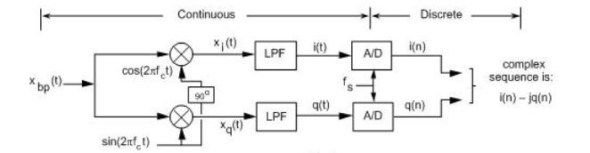
See this jupyter notebook for an introduction to the idea.
Now demonstrate IQ processing in GNU Radio. We can demonstrate this at much lower frequencies as well. Set the sample-rate to 48kHz. Create 2 tones(cosine signals), one at 8kHz, one at 12kHz. Create your LO at 10kHz, one a cosine and one a sine.
Try using the two signals independently, and added together, this is the overall ‘signal’. Now multiply this signal by the cosine and the sine “LO’s”. This now will become your IQ signal. Pass these signals into GNU Radio’s “float to complex” block. The cosine-mixed signal forms the real part, and the sine-mixed signal forms the imaginary part. This can then be passed into a sink.
Add different sinks along the way, looking at just the cosine (“I”) or sine (“Q”) multiplied signals. With just the single incoming tone, demonstrate that you can in fact recover it after mixing. Do we need a filter? Where? Add one if needed.
5.2. Fast Fourier Transforms (FFT)
The Discrete Fourier Transform for N samples is given by:
\[X[k] = \sum_{n=0}^{N-1} x[n] \cdot e^\frac{-2\pi kn}{N}\]Direct DFT evaluation requires \(N^2\) complex multiplications and N(N-1) complex additions. Eliminating trivial operations, such as multiplication by 1, saves \(O(N)\) operations. Multiplications are particularly expensive computations.
Fast Fourier transform algorithms drastically reduce the computational complexity. The radix-2 Cooley–Tukey algorithm is a widely used FFT algorithm. It computes the same result using \(\frac{N}{2}log_2(N)\) complex multiplications and \(Nlog_2(N)\) complex additions. These counts ignore simplifications such as multiplication by 1.
Read C. S. Burrus’s notes on FFT algorithms, including the Cooley-Tukey method and references for further study.
5.2.1. 8 Point Fast Fourier Transform [OPTIONAL]
The DFT implemented through a Cooley-Tukey Decimation in frequency FFT algorithm has the flowgraph shown below.
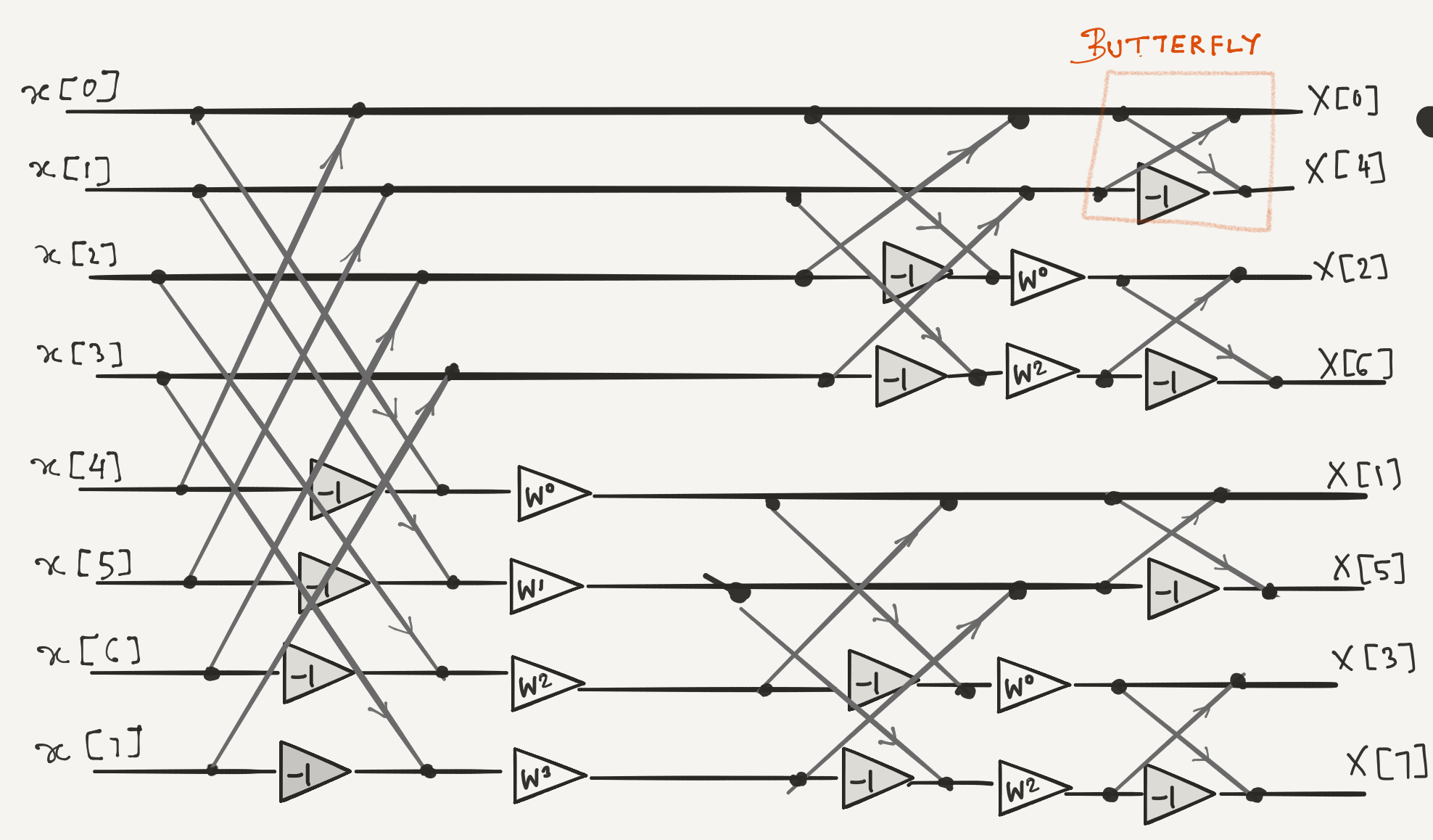
Build this in GNU Radio using constant multipliers and adders. Use \(W^{i} = e^{\frac{-2\pi k i}{8}}\). Are the outputs the valid frequency-domain results?
5.3. Fourier Analysis in Radio Astronomy: A Spectrometer
You now have the tools necessary to create the digital signal processing for a Spectrometer for a radio telescope. A spectrometer:
- Separates incoming radio signals into frequency components (cosine amplitudes and phases at each frequency)
- Measures the power in each of the cosine waves.
- Integrates (Averages) to get get a more precise measurement of the power at each frequency.
Use GNU Radio to create the signal processing chain to achieve this. Use an osmocom airspy source. Use an FFT to separate frequency components.
5.4. The Spectrometer’s purpose
A spectrometer records and measures a signal’s spectral content. That signal may come from an astronomical radio source. Specifically, a spectrometer measures the power spectral density (PSD, measured in units of \(W\,\mathrm{Hz}^{-1}\)) of a signal. Spectral analysis reveals properties of radio sources and intervening material, such as galactic neutral hydrogen. The Power Spectral Density is given by the Wiener-Kinchin theorem for wide sense stationary signals as:
\(S_{xx}(\nu) = \int^{\infty}_{^-\infty}r_{xx}(\tau) e^{-2\pi i\nu\tau}d\tau\) \(r_{xx}= E[x(t)(x(t-\tau)]\)
and in the fourier domain
\[S_{xx}(\nu)=E[|X(\nu)|^2]\]E[] stands for the expected value i.e. the mean
Spectrometers can estimate \(S_{xx} (k)\) in two ways. One method forms the autocorrelation, then takes its Fourier transform. The other forms frequency-domain X(k), then evaluates \(S_{xx} (k)\). These are Autocorrelation Spectrometers and Fourier Transform Filter banks respectively.
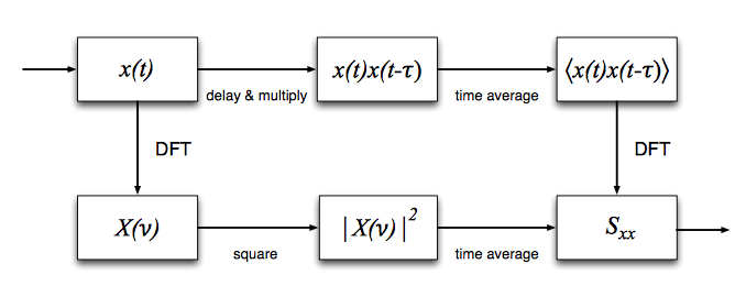
The one we made above is a Fourier transform filter bank. A filter bank is simply an array of band-pass filters, designed to split an input signal into multiple components . A spectrometer is referred to as a analysis filterbank where the output of each filter is squared and averaged.
5.5. The Window Field in the GNU Radio FFT block
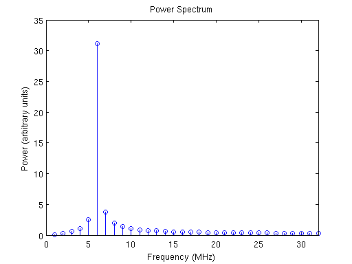
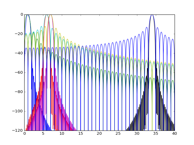
The spectrometer we constructed effectively works as a array of band-pass FIR filters. If you recall FIR filters their design involves something called window-functions designed to optimize the filter response. The Discrete Fourier transform as it were uses the rectangular window function across each frequency channel. The response is non-ideal leading to spectral leakage i.e. the signal showing up in neighboring frequency channels. The example below demonstrates DFT leakage. A 5.1 MHz tone is sampled at 128 MHz and transformed using 64 points. It appears with varying strength in every output frequency bin.
This can be improved by using better windowing functions to properly define the frequency channel. Below are some commonly used windowing functions.
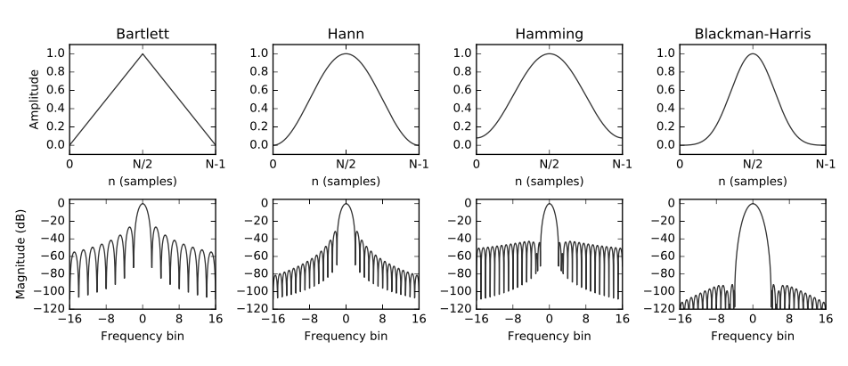
Main-lobe width and sidelobe attenuation determine how clearly frequency channels are defined. The figures below illustrate the difference. The second plot compares window responses across frequency bins. Boxcar windows have higher sidelobes; the Hann window has lower sidelobes.
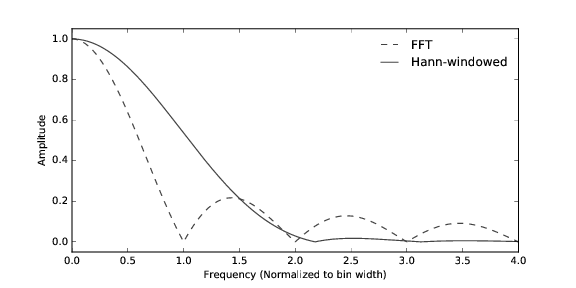
Change the FFT block’s window field in your spectrometer flowgraph. Observe how each window changes the response to a sinusoidal tone.
5.6. Spectral Leakage and Polyphase Filter Bank (PFB)
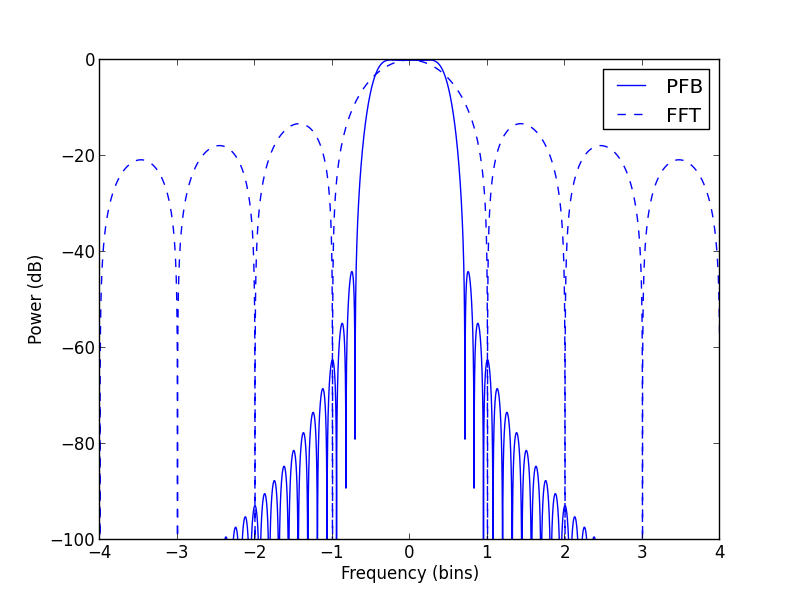
Despite the appropriate windowing, spectral leakage persists, moreover there is something called a scalloping loss. Scalloping loss occurs between frequency-bin centers because each bin’s frequency response is not flat.
The polyphase filter bank (PFB) technique is a mechanism for alleviating the aforementioned drawbacks of the straightforward DFT. The PFB provides a flat channel response and strongly suppresses signals outside the band, as shown below.
“Rather than taking an N-point transform directly, read N x P = M samples. Multiply them point by point by a window function (the data is ‘weighted’). As mentioned before, the shape of the window function determines the shape of the single-bin frequency response. We want each bin’s frequency response to resemble a rectangle. We therefore choose its Fourier transform pair, the sinc function, as the window. After multiplication, split the data into P subsets containing N samples each. Add the subsets point by point. This array is then passed to a regular DFT routine to get an N-point transform that exhibits less leakage. This method is presented graphically below”1
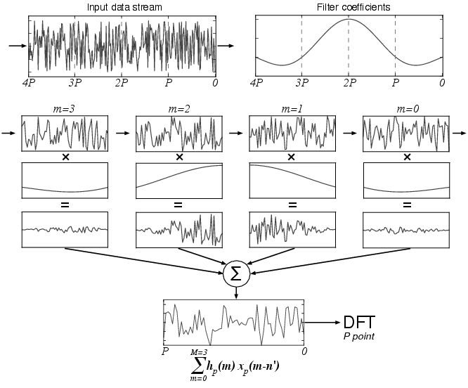
The same process, mathematically:
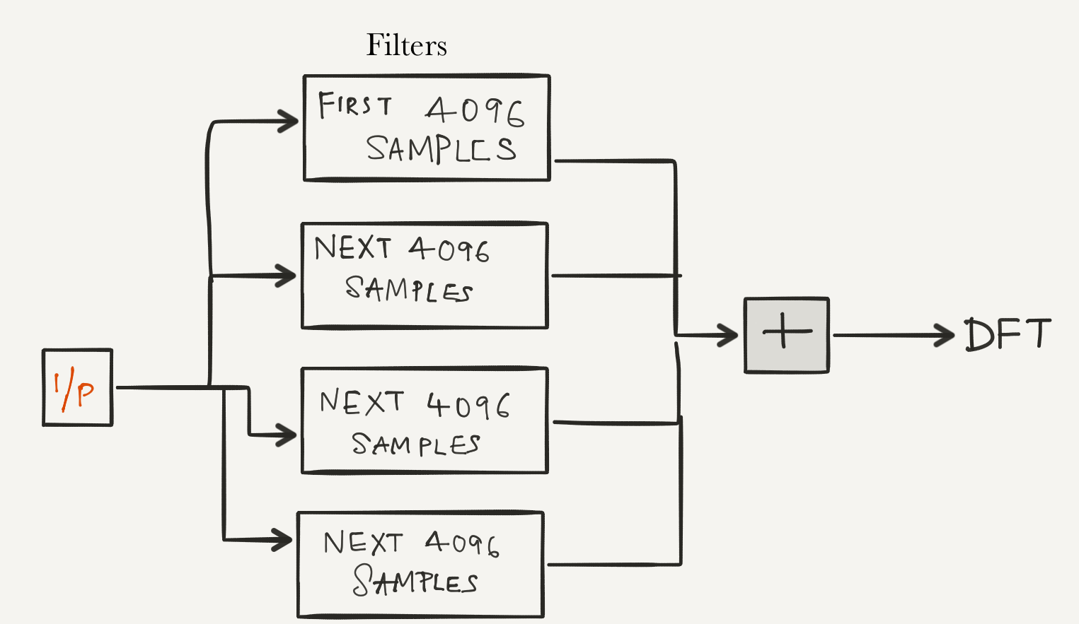
\[y(n) = \sum_{p=0}^{P-1} x(n + pN) h(n+pN)\]Where the sub-filter coefficients \(h(n + pN)\) correspond to what are called P-tap ‘polyphase sub-filters’. These N polyphase sub-filters and the following DFT stage form a ‘polyphase filter bank’ (‘PFB’). A realization of this filter bank is shown below:
5.7. Final Upgrade: PFB Spectrometer
Add the polyphase filters to your spectrometer just before taking the FFT. Refer to the diagram above, the dotted squares are simply band-pass FIR filters. Use a hann/hamming window.
The polyphase filter can be realized by implementing following flowgraph:
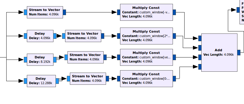
The constant multiplier blocks are sections of the filter window as seen the diagram detailing the process above. The filter window is designed by using import block to import numpy and assigning three constant variables as:
- sinc_sample_locations
np.arange(-np.pi*4/2.0, np.pi*4/2.0, np.pi/vec_length) - sinc
np.sinc(sinc_sample_locations/np.pi) - custom_window
sinc*np.hamming(4*vec_length)Now
custom_windowcontains the window coefficients, or taps. Use them for multiplication one vector of samples at a time. The constants in the constant multiplier blocks from the top to bottom are as follows:custom_window[-vec_length:] custom_window[2*vec_length:3*vec_length] custom_window[vec_length:2*vec_length] custom_window[0:vec_length]
5.8. Saving Data
Save the spectrometer data for science! (Use File Sink)
NOTE: Our Low Noise Amplifier (LNA) needs to be powered to actually work. Enable the Airspy’s bias tee by setting bias=1 in the osmocom source block’s device arguments:
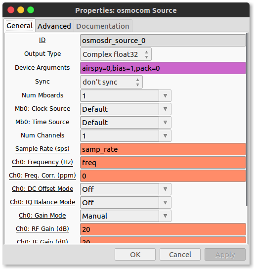
Image Credits
- The windows, the two types of spectrometers,fft vs hann response https://arxiv.org/pdf/1607.03579.pdf
- The PFB flowgraph, spectral leakage demo, https://casper.berkeley.edu/wiki/The_Polyphase_Filter_Bank_Technique
- IQ diagram https://www.dsprelated.com/showarticle/192.php