
2. Software Defined Radio - Hardware
In Lab 1 we learned how to work around GNU Radio Companion (GRC) and simulate signals and instruments. We shall now step into the real world with real signals.
2.1. Introduction
A “simplified” diagram of the device which we shall be using is shown below:
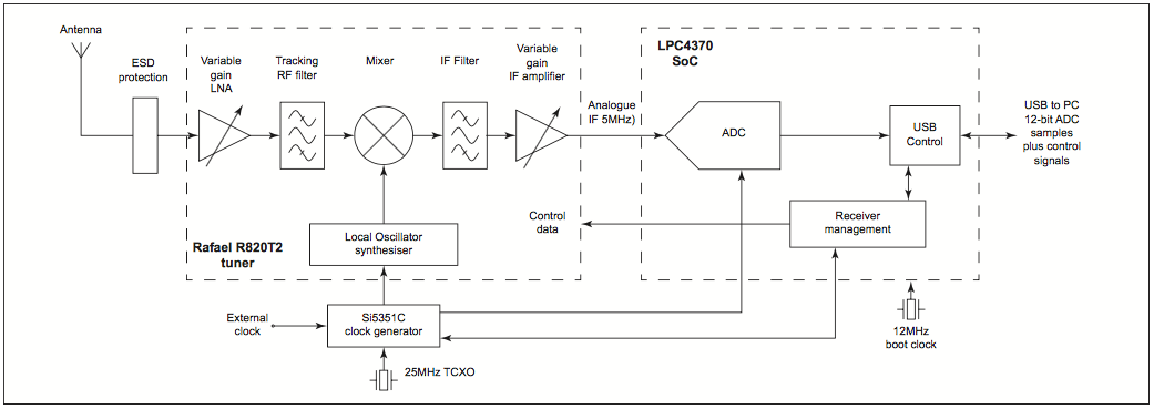
Simplifying this further for a general SDR hardware including the energy conversions:
(EM Waves)))) >-(Antenna)–>(Amplifier)—>(Local Oscillators + Filters)–>(Analog to Digital Convertor)–>(networking control: usually USB)—>[Computer]
Radio Waves excite electrons in the antenna and induces a current. The frequencies the antenna is most sensitive to is determined by the geometry of the antenna’s design. The electric current is then initially amplified a bit. Use a “Low Noise Amplifier” to minimize noise added by local electronics to the antenna signal. Processing at a fixed frequency improves receiver performance. A local oscillator (LO) enables this conversion. It is an electronic oscillator used with a mixer to change the frequency of a signal. This conversion is called heterodyning. It produces the sum and difference of the input and local oscillator frequencies. The desired frequency is then filtered out and if required amplified again. Finally, digitize the signal and send it to the computer. Our GNU Radio code can then process it.
2.2 Frequency Correction of the SDR Dongle
The hardware is well made, but a precision clock is quite expensive. The frequency the “tuner” tunes to may be slightly off from the actual frequency it is tuning to. We can correct for that in the software. For high-end SDR dongles this correction is virtually non existent but some low-end dongles have higher deviations!
We can transmit a signal using a known and reliable tone. Then we use our receiver set up with gqrx to see the signal. If the incoming signal is exactly at the expected frequency then the internal clock is working well. Otherwise, open gqrx’s input controls tab. Adjust freq. correction until the peak reaches the correct position.
This value will be different for all dongles. It also changes with the temperature of the dongle. It is interesting to watch this change as the dongle warms up. Note your value for future purposes.
2.3. GNU Radio FM
We used gqrx in section 1.2 to listen to FM now we shall code our own radio using GRC!
2.3.1 Signal Modulation
Modulation is a process of mixing a signal with a sinusoid to produce a new signal. Consider a signal represented by the function:
\[f(t) = A \sin(\omega t + \phi).\]This sinusoid has 3 variables that can be altered ti change the function f(t). The first term, A, is called the magnitude, or amplitude of the sinusoid. The next term, \(\omega\) is known as the frequency, and the last term, \(\phi\) is known as the phase angle. We can encode our message in either of these three parameters.
The sinusoidal signal that is used in the modulation is known as the carrier signal, or simply “the carrier”. The signal modulating the sinusoidal carrier is the “data signal” or “message signal”.
Some data signals are unsuitable for direct transmission. Modulation can produce a signal better suited to transmission.
It follows from above we encode in the above three variables. Consequently, we have 3 basic types of analog modulation:
- Amplitude Modulation
- Frequency Modulation
- Phase Modulation
2.3.1.1 Amplitude Modulation
For our discussion of amplitude modulation consider a carrier wave of frequency \(f_c\) and amplitude \(A\) given by:
\[c(t) = A \cdot \sin(2 \pi f_c t).\]Let \(m(t)\) represent the modulation waveform. Use a sine wave at \(f_m\) for modulation. Choose a frequency, such as audio, much lower than \(f_c\):
\[m(t) = M\cdot \cos(2 \pi f_m t + \phi),\]where \(M\) is the amplitude of the modulation. If \(M>1\) then overmodulation occurs and reconstruction of message signal from the transmitted signal is more difficult. Amplitude modulation results when the carrier \(c(t)\) is multiplied by the positive quantity \((1+m(t))\):
\[y(t) = [1 + m(t)]\cdot c(t) \\ \ \ = [1 + M\cdot \cos(2 \pi f_m t + \phi)] \cdot A \cdot \sin(2 \pi f_c t)\]Using trigonometric identities, \(y(t)\) can be shown to be the sum of three sine waves:
\[y(t) = A \cdot \sin(2 \pi f_c t) + \frac{AM}{2} \left[\sin(2 \pi (f_c + f_m) t + \phi) + \sin(2 \pi (f_c - f_m) t - \phi)\right]\]The modulated signal has three components. The carrier \(c(t)\) is unchanged. Two sine-wave sidebands lie just above and below the carrier frequency \(f_c\).
Demodulation or extracting the message from the carrier involves simply filtering out the carrier signal. We can build an AM receiver in GNU Radio. However, our SDR dongle tunes only from about 20 MHz to 1800 MHz.
2.3.1.2 Frequency Modulation
The message is encoded in the carrier’s frequency: \(x(t) = a \sin (f(t)t + \phi)\). Let the message signal be \(x_m(t)\) and the carrier be \(x_c(t) = A_c \cos (2 \pi f_c t)\). Here, \(f_c\) is the carrier frequency, and \(A_c\) is its amplitude. The modulator combines the carrier and message to produce the transmitted signal
\[\begin{align} y(t) & = A_c \cos \left( 2 \pi f(t) t \right) \\ & = A_{c} \cos \left( 2 \pi \left[ f_{c} + f_{\Delta} x_{m}(t) \right] t\right)\\ & = A_{c} \cos \left( 2 \pi f_{c} t + 2 \pi f_{\Delta} x_{m}(t) t \right) \\ \end{align}\]where \(f_{\Delta}\) is the sensitivity of the frequency modulator which adjusts how much bandwidth is used for the signal.
2.3.2 Let’s Make our FM Radio
Demodulation extracts the message encoded in the sinusoid’s changing frequency. That can be achieved by “fast” differentiating the sine wave, treating the message as a constant. Consider the following:
\[x(t) = a \sin (f(t)t + \phi) \\ \frac{d x(t)}{dt} = af(t) \cos(f(t)t + \phi) \\ \ \ \ = A(t) \cos(f(t) + \phi)\]For the FM signal
\[y(t) = A_c \cos \left( 2 \pi f_c t + 2 \pi f_{\Delta} x_{m} (t) t \right) \\ \ \ \ = A_c cos ( \theta(t) )\] \[\begin{align} y'(t) & = -A_c \theta ' (t) \sin(\theta (t) ) \\ & = -2 \pi A_c ( f_c + f_{\Delta} x_m(t) ) \sin (\theta (t)) \end{align}\]The converted signal is \(y(t) = [1 + m(t)]\cdot c(t)\). This is an AM signal. We can easily demodulate this AM signal by filtering out the AM “carrier”. It follows the following flow:
| FM —-> | Differentiator | —-> | Envelope Detector | —-> Signal |
A similar operation can be achieved in GNU radio using the following flow:
| FM —> | Filter out the signal of interest | —> | Resample Signal | —> | Quadrature Demodulator | —> | Lowpass Filter | —> Audio Signal |
The quadrature demodulator handles complex input, so it uses a method other than differentiation. Its output is still proportional to changes in input frequency. (That GNU Radio block actually has a good explanation of the math in the description. )
Hints:
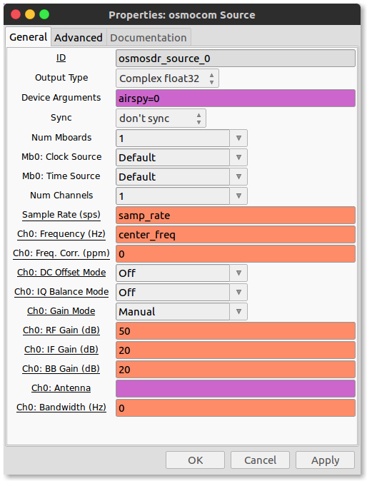
Source: Since we are using a hardware source we have to use the appropriate block. Search for the osmocom Source block. The Device arguments should be airspy=0. NOTE: The Sample rate supported by this dongle is either 2.5 MHz or 10 MHz. We shall set our samp_freq variable to 2500000. The Ch0: Frequency (Hz) is the frequency you want to tune to.
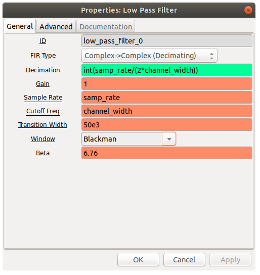
Low Pass Filter: This filters out all the frequencies apart from the one we want to tune our radio to. Note that I have another variable called channel_width which is equal to 200e3. It is to filter out at a data rate 200kHz.
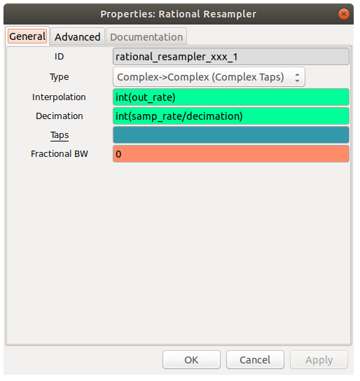
Resampling Signal: Use the ‘Rational Resampler’ block. Resample the signal such that the frequency of the signal is a multiple of out output frequency. The output sample rate (‘out_rate’) matches the sound card’s input rate: 48 kHz for audio playback. The output frequency should still be near to the bandwidth of the message i.e. 200kHz. 192kHz ie ‘out_rate’ is the closest multiple of 48kHz to it. As noticed on the screen shot here is a new variable ‘decimation == int(samp_rate/(2*channel_width))’
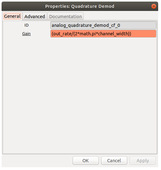
Quadrature demodulation extracts the changing frequency component, which carries the audio. In the quad demod block, set gain to ‘(out_rate/(2math.pichannel_width))’
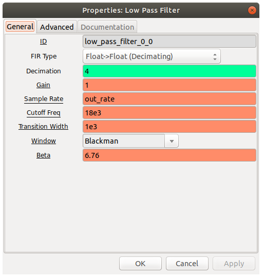
Lowpass Filter: Set the cutoff to 18 kHz (near the upper limit of human hearing). Set decimation to reduce the 192 kHz input to the sound card’s 48 kHz sample rate.
Play audio from an audio sink
Lets capture some sweet tunes!
2.4. Fun SDR/GNU Radio things
- AM Radio! (see above)
- Narrow Band FM ( same are FM but a narrower filter passband)
- Listen to and get airplane ADS-B data To check it out on your own get this software: dump1090
- Listen to HAM radio chatter ( usually amplitude modulated )
- EMS and police and local services radio. local scanners and frequencies
- WeatherFAX. Get latest images of weather data from naval bases! http://www.rtl-sdr.com/receiving-weather-rtty-rtl-sdr/
- Get satellite data: receive and decode live images of Earth. These satellites transmit at the following frequencies:
- NOAA 15: 137.6200 MHz
- NOAA 18: 137.9125 MHz
- NOAA 19: 137.1000 MHz
- If transmitted nearby get a newspaper over the radio!
- Decode high definition radio with
nrsc5 - Build your own radio astronomy observatory! ( ok we are totally doing that!)