
1. Introduction to GNU Radio and Signals
This page shall guide you through our primary tool – GNU Radio. GNU Radio is very popular and robust Software defined radio package. It is open source and is relatively very easy to use. All “coding” is done using flowgraphs comprised of interconnected Digital Signal Processing (DSP) blocks. The package includes commonly used blocks. You can also program your own.
- 1. Introduction to GNU Radio and Signals
1.1. Installing GNU Radio
1.2. GQRX - It’s cool
GQRX is an application written using GNU Radio. It acquired data from the dongle and has a set of preset options to manipulate said signals. It can even store raw data for custom decoding. Install it with:
sudo apt install gqrx-sdr
Plug the dongle into USB. Check that the computer detects it by typing airspy_info. If we installed all software correctly it should return information about the dongle and no errors. If everything is in order the type in terminal:
gqrx
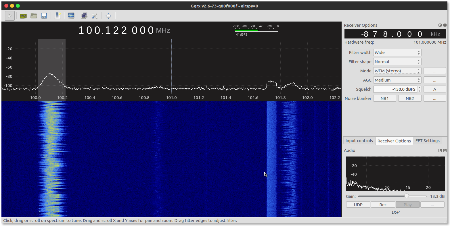
It will open a window that looks like this.
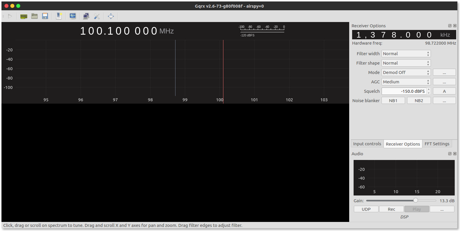
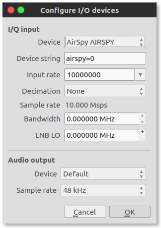
On first use, the hardware or IO settings window should open automatically. It should also detect the dongle. If not chose AirSpy AIRSPY from the drop down.
Otherwise you can open it by clicking on the “circuit board” icon next to the play triangle. The I/O device settings should look like this:
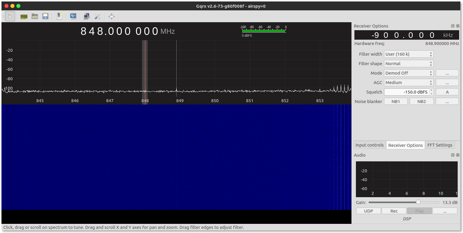
Once it is all in order click play. The window should show the spectrum as such:
Hit play. Change the frequency to 100 Mhz. Notice the bright bands on the waterfall and the peaks, these are local FM stations
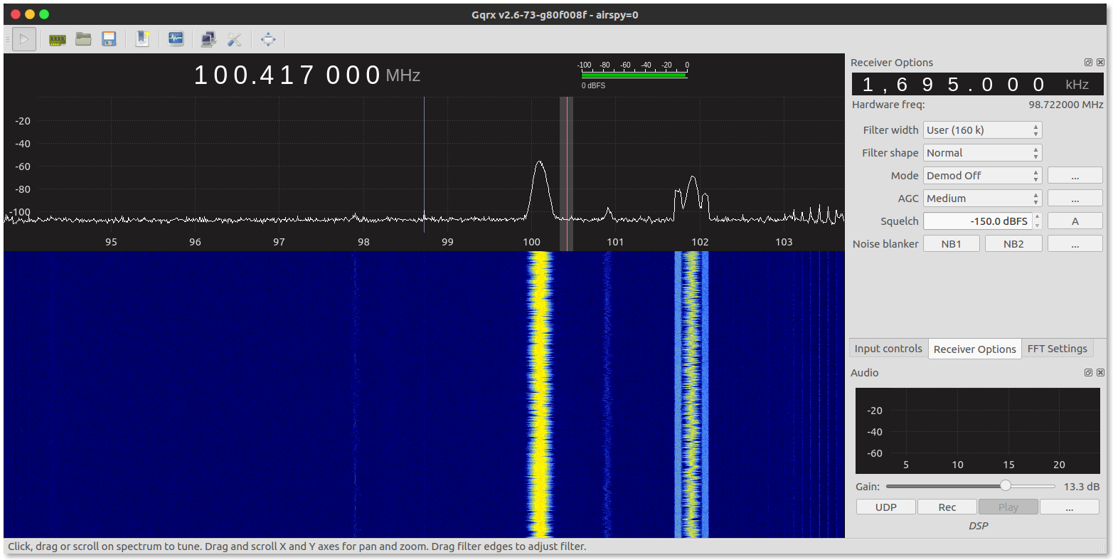
Since the sample rate is very high (a feature of this particular hardware). We click on the “circuit board” button again and change input rate 2500000 (from the drop down). In the receiver options at right, set Mode to WFM (wideband FM). You can now listen to broadcast radio on your computer.
We can use this application to receive even decode to all kinds of signals from 24 – 1800 Mhz. Check out Section 2.4
1.2.1. Getting Started with GNU Radio
As mentioned earlier, gqrx has GNUradio as its engine. We can start developing using this tool right away by typing gnuradio-companion in the terminal:

This opens GNU Radio Companion (GRC):
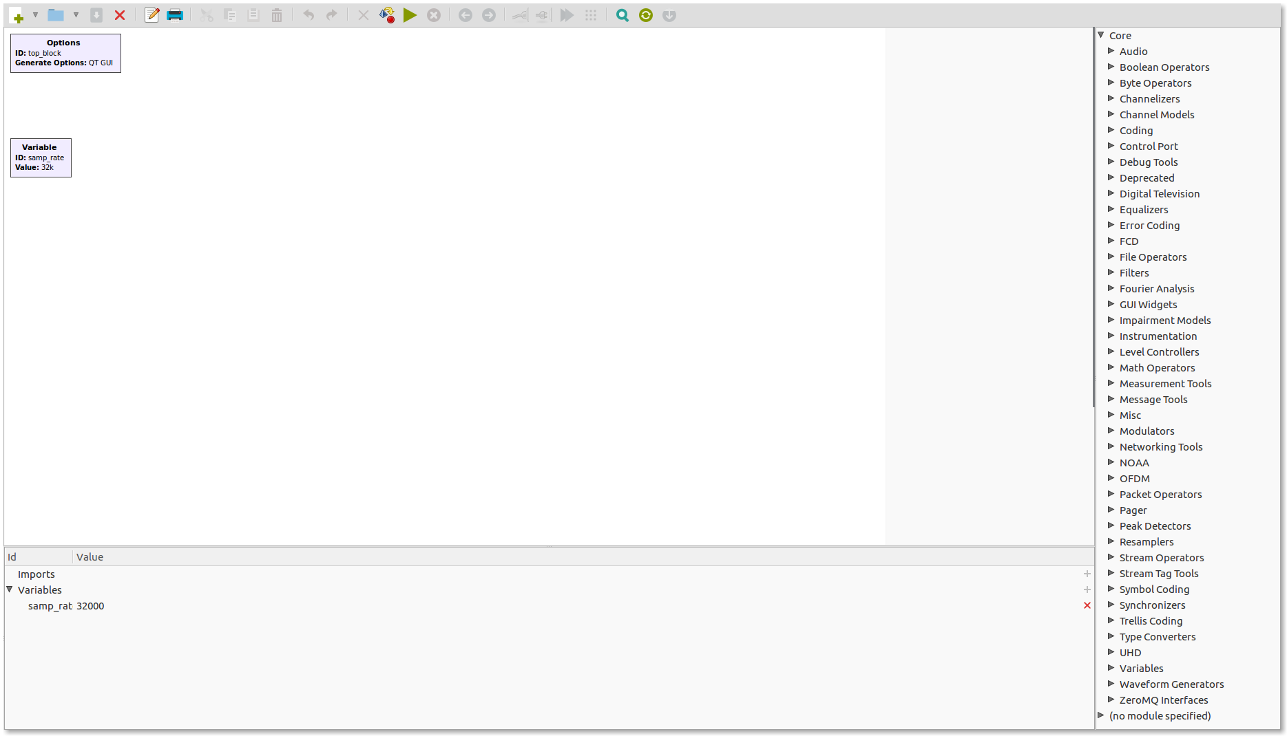
The “Options” block at the upper left controls general flowgraph settings. These include title, author, graphical interface, result displays, and canvas size. Right-click the block and choose Properties, or double-click it. This opens its configurable parameters. The “Variable” block below Options defines values used throughout the flowgraph. An example is the sample rate, \(F_s = 32000 Hz\)
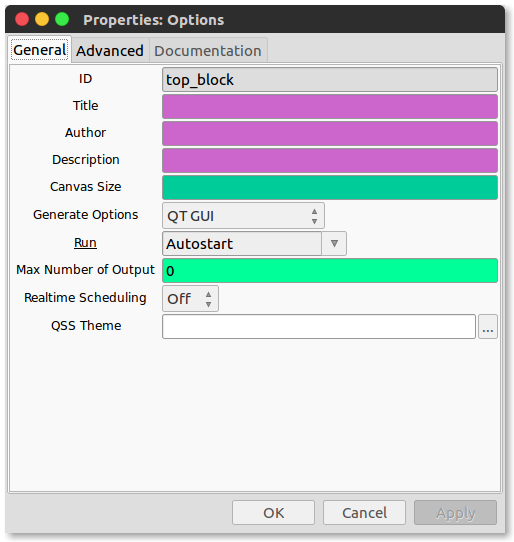
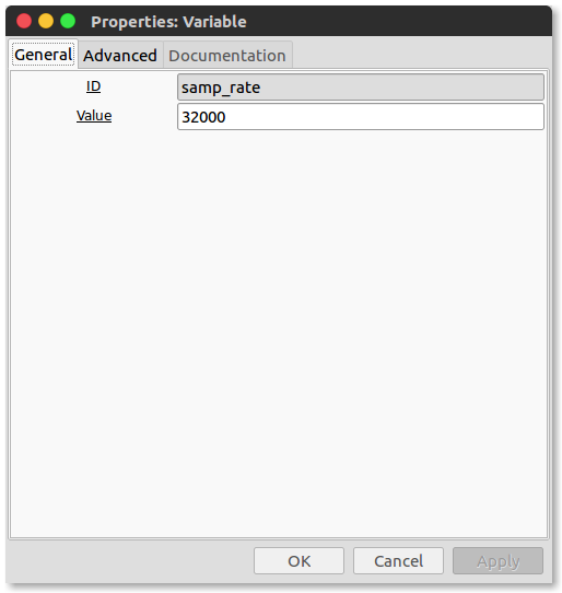
Every GRC window has these two very basic blocks. The white space is called the GRC canvas.
1.3. Let’s get Familiar
On the right side of the window is a list of the block categories that are available. Click on a triangle next to a category to see what blocks are available in that category. We will look for the waveform generator category to look for the signal source block. Alternatively, we can click on the magnifying/looking glass to the top right and search for the block we need. We will add the signal source block to the canvas by double clicking on signal source
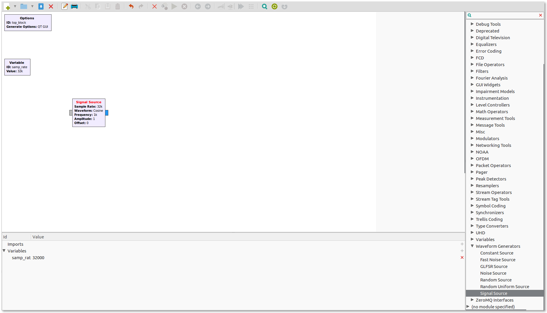
To move a block, hold the left mouse button over it and drag it to the desired location. You can also rotate blocks by right-clicking on them and then clicking either “Rotate Counterclockwise” or “Rotate Clockwise”. Blocks can also be temporarily disabled by clicking on “Disable”, which is useful for debugging and what-if questions. The rearranged blocks with the options for the “Signal Source” visible are shown next.
Aside
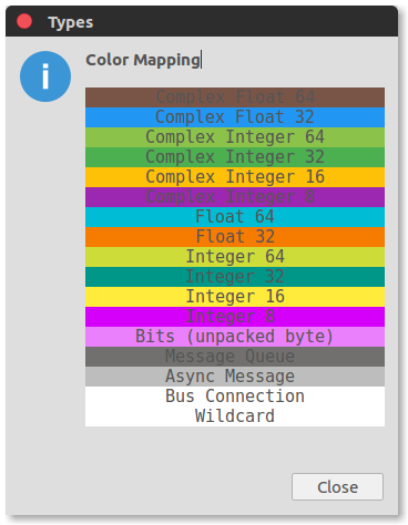
The “Signal Source” block has a gray port on the left and a blue port on the right. Port colors identify the data type generated by an output or accepted by an input. The most common data types that we will use are:
- Blue for complex-valued 32-bit floating point data samples (32 bits for each, real and imaginary part).
- Orange for real-valued 32-bit floating point data samples
- Blue-Green for real-valued 32-bit (long) integer data samples
- Yellow for real-valued 16-bit (short) integer data samples
- Magenta for real-valued 8-bit (byte) integer data samples
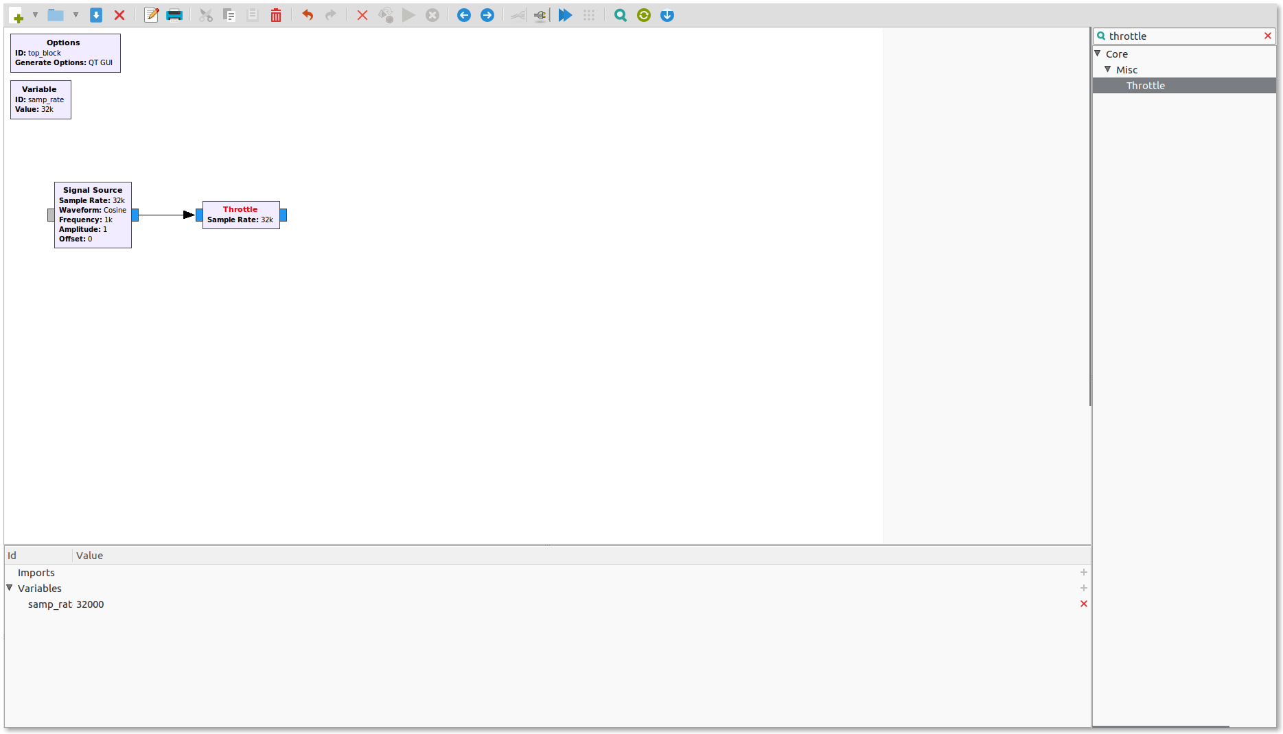
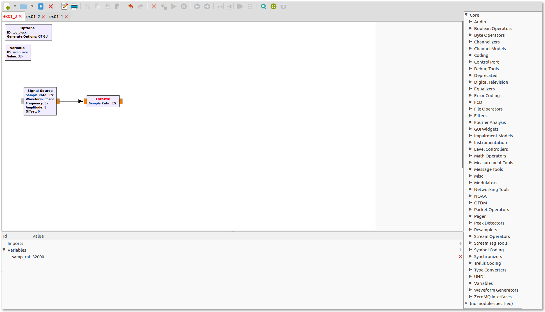
GNU Radio processes large datasets in real time using streams. This differs from array-processing environments (like Matlab). Each signal-processing block has its own scheduler and execution thread. It runs as quickly as CPU capacity, data flow, and buffer space permit. A hardware source or sink can set the overall rate. Examples include 44100 samples/sec for audio and 10 Msamples/sec for an SDR interface. Software-only sources and sinks need a software timing constraint. Without one, a signal generator feeding a display could exceed the intended sampling rate. A special “Throttle” block that we will frequently encounter is used for this purpose. The figure below shows a “Throttle” block connected to the output of the “Signal Source” that we placed earlier. Click an output port, then the destination input port. This wires the two blocks together. The connected ports must have matching data types (i.e., the same color). If they are of different types, then the arrow of the connection will be red instead of black. The red “Throttle” label indicates a problem with that block in the flowgraph. Possible problems include missing parameters, undefined values, or missing port connections, as shown above. Fix any red arrows or labels before running the flowgraph.
1.3.1. A Cosine Waveform generator
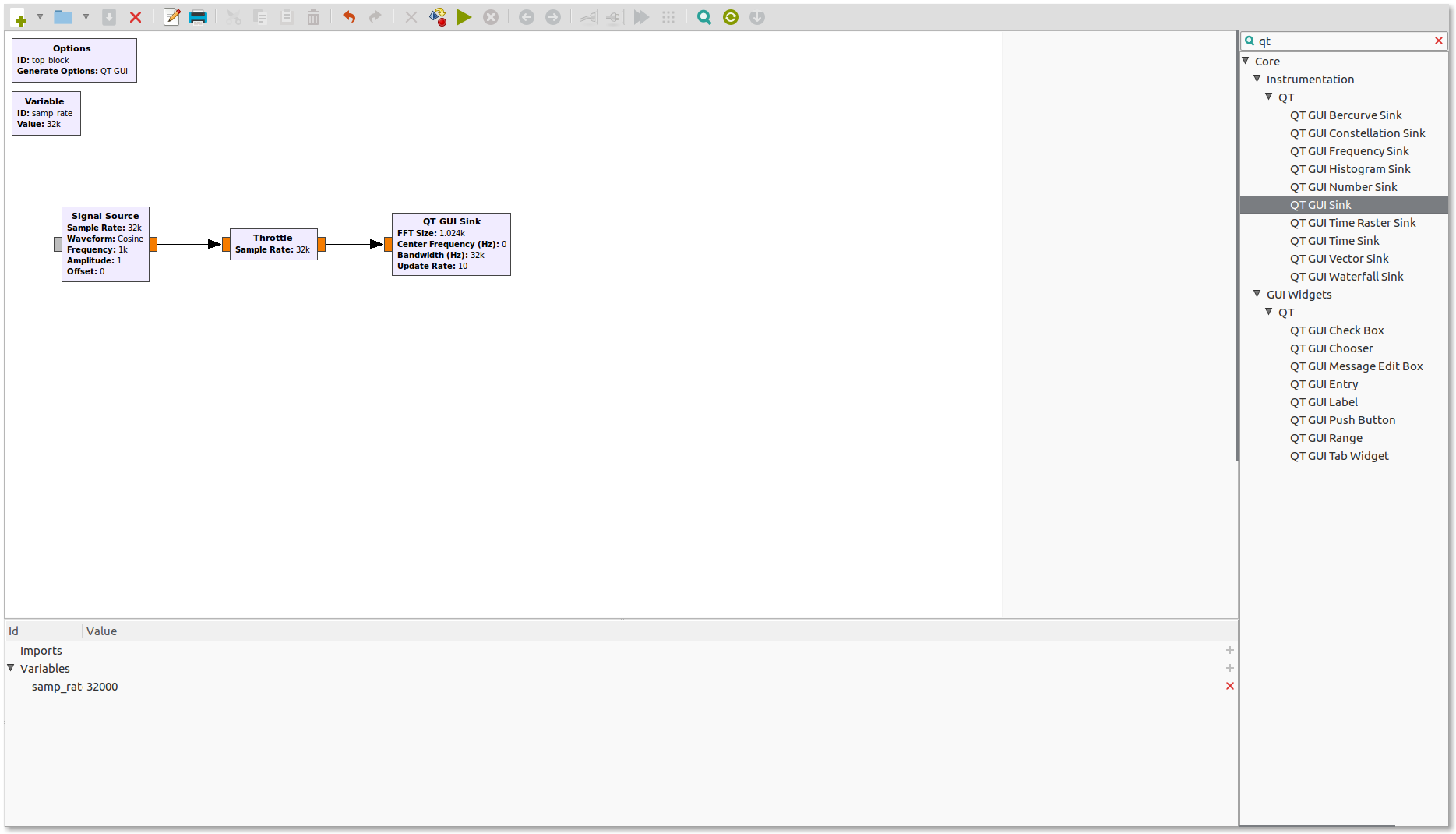
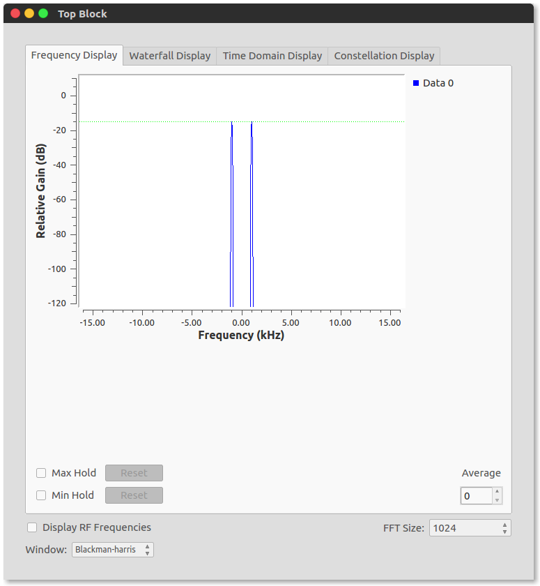
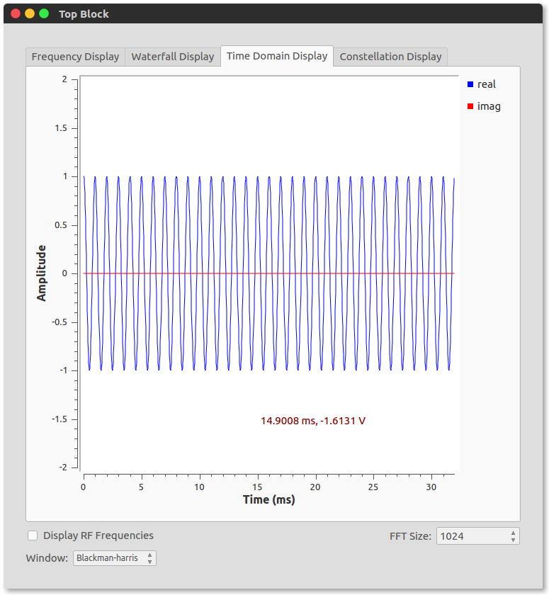
First, generate a real cosine signal at 1000 Hz, the “Signal Source” default. Display it in both time and frequency domains. We start from a flowgraph which consists of a “Signal Source” connected to a “Throttle”. Double-click Signal Source to open its Properties. Under “Output Type”, change “Complex” to “Float”, as shown below. This makes the output real-valued. Then choose “QT” under “Instrumentation” (or just simply search for “QT GUI Sink”) and double-click on “QT GUI Sink”. This block displays the input waveform in both time and frequency domains. Change the data “Type” from “Complex” to “Float” and connect the input to the output of the “Throttle” block. Save the flowgraph, e.g., as ex01_1.grc
Run the flowgraph using the green triangle above the canvas or “Run” in the menu bar. You can choose between the “Frequency Display” and the “Time Domain Display” tabs as shown below. Drag the cursor to zoom into a rectangle. Increase the FFT size to 4096 or 8192. Try windows such as “rectangular” and “Kaiser”. Observe the changes, especially in the Frequency Display. The Frequency Display shows power spectral density (PSD). This is proportional to the squared magnitude of the Fourier transform.
1.3.2. A Cosine Waveform Generator with Variable Frequency and Sound
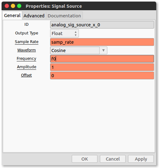
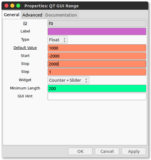
We can start from the ex01_1.grc flowgraph from our first exercise. Under “GUI Widgets” and “QT” select “QT GUI Range”. Double- click on the block so that you get to see its Properties. Change the “ID” from variable_qtgui_range_0 to f0. For the “Default Value” enter 1000. For the “Start” and the “Stop” values enter -2000 and 2000, respectively. Next we double-click on the “Signal Source” block and change the “Frequency” entry from 1000 to f0. The respective windows look like below:
To add a sound output, select “Audio” and then double-click on “Audio Sink”. Connect the “Audio Sink” input to the “Throttle” output. Keep the default “Sample Rate” of samp_rate (32000 samples/sec).
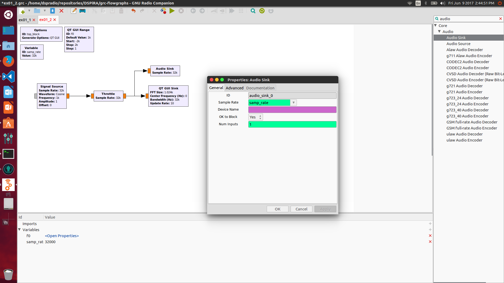
Save the flowgraph, e.g., as ex01_2.grc. Run the flowgraph to adjust “Signal Source” frequency with a slider from -2000 to +2000 Hz. You will hear the corresponding sound. Choose either the “Frequency” or “Time Domain” graph.
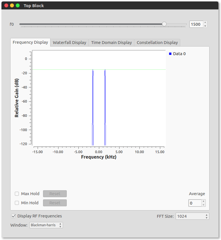
Difference between \(+ve\ \&\ -ve\) frequencies?
1.3.3. A General Waveform Generator
This subsection extends the previous exercise with more GNU Radio Companion features. Let us begin by changing ex01_2.grc flowgraph by removing the “Audio Sink” and the “QT GUI Sink”. Save this new flowgraph as ex01_3.grc
Build a generator for real “Cosine”, “Rectangular”, and “Triangular” waveforms. Make the frequency and dc offset adjustable. To this end we need “QT GUI Range” blocks and a “QT GUI Chooser (from “GUI Widgets” and “QT”). Find “QT GUI Time Sink” and “QT GUI Frequency Sink” under “Instrumentation” and “QT”. Connect both to the “Throttle” output. Change the input type of the Sink blocks from “Complex” to “Float”. The flowgraph should look like this:
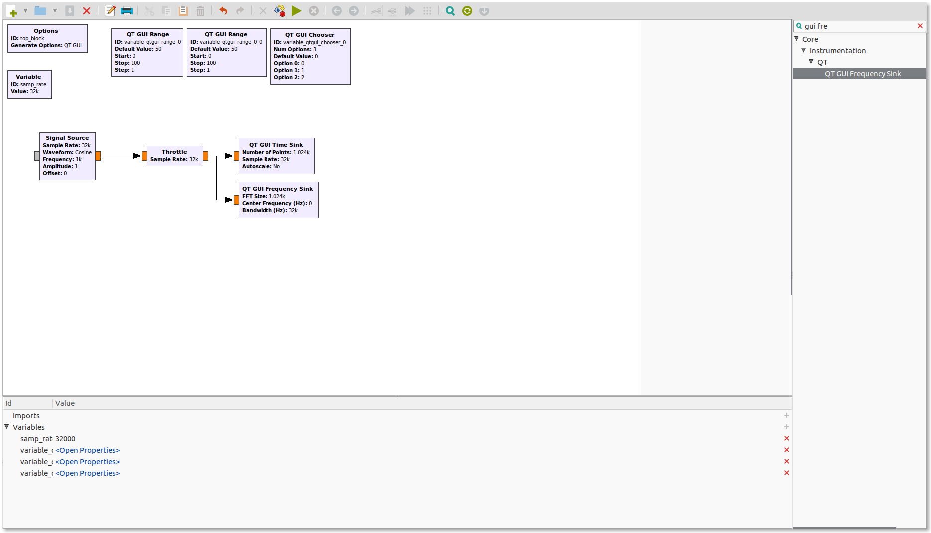
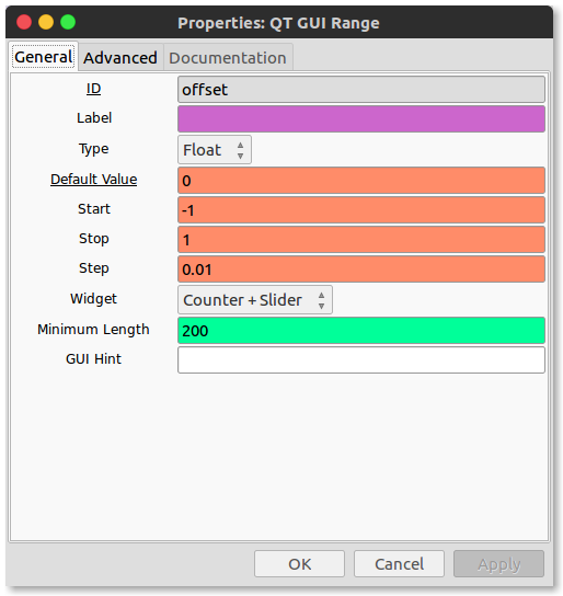
Double-click the second “QT GUI Range” to adjust waveform offset. Change its “Properties” as shown below:
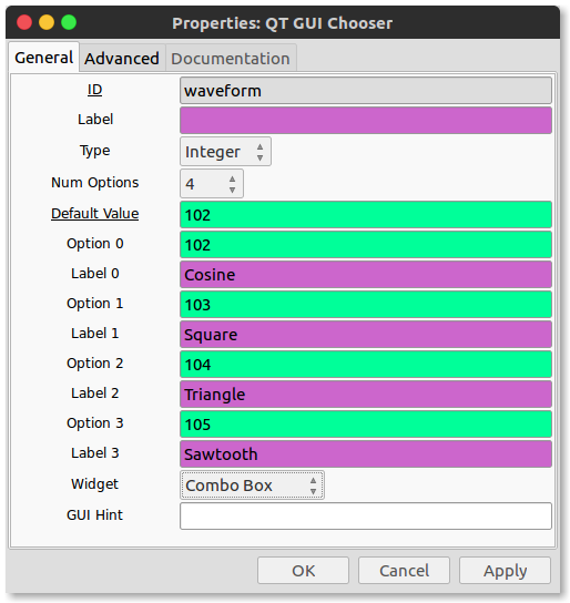
Next, double-click on the “QT GUI Chooser” that will be used to select different waveforms. The integer codes are 102 for “Cosine” and 103 for “Square”. Use 104 for “Triangle” and 105 for “Sawtooth”
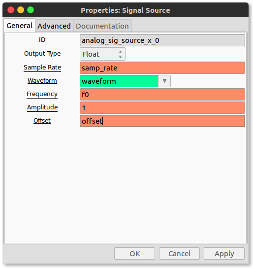
Finally, double-click on the “Signal Source” block and modify the “Properties” to look as follows.
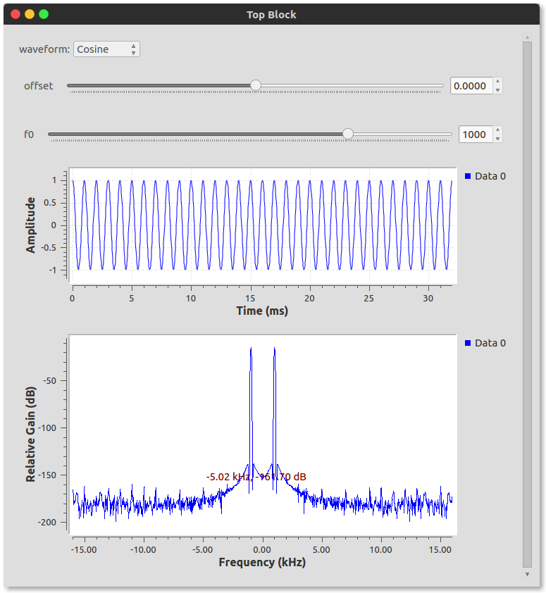
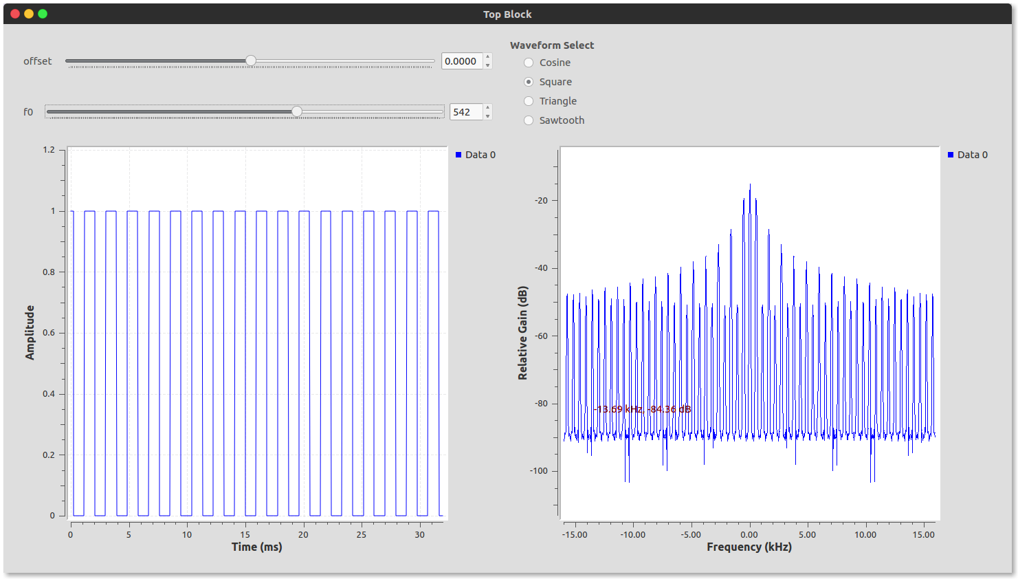
Double click on the sinks and change to autoscale property to “Yes” respectively. Click the green triangle above the flowgraph or click on “Run” and “Execute” in the GRC menu bar. The output is as below:
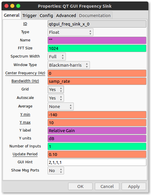
Set grid positions in each block’s “GUI Hint” field. These positions arrange sliders, choosers, and time or frequency sinks in the interface. A grid positioning argument is a list of four integers of the form
row, column, row span, column span
If the “GUI Hint” entry is left blank, then the graphical elements are stacked vertically on top of each other. Otherwise, they are placed in the specified row and the specified column, spanning row span rows and col span columns. Note that rowspan >= 1 and colspan >= 1 are required.
| (0,0) | (0,1) | (0,2) | (0,3) |
|---|---|---|---|
| (1,0) | (1,1) | (1,2) | (1,3) |
| (2,0) | (2,1) | (2,2) | (2,3) |
We shall rearrange our signal generator with the following GUI Hints
| Offset Slider (0,0,1,1) | Waveform Selector (0,1,2,1) |
|---|---|
| Frequency Slider (1,0,1,1) | ” |
| Time Display (2,0,1,1) | Frequency Display (2,1,1,1) |
The GUI hints are updated as seen the following dialog boxes:
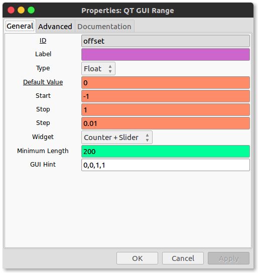
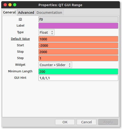
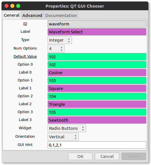
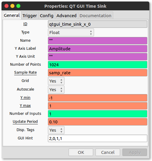
This give the following Output:
1.4. GNU Radio and Python
GNU Radio is written in python and the final code that does the magic is all in Python. Python is very powerful programing language known for its readability and versatility. The flow graphs created in GNU radio companion are converted into a Python script. All the predefined blocks are written in Python and/or C. One can make their own GNU Radio blocks by coding in Python or C. For more detail, read the GNU Radio Python guided tutorial
1.4.1. Arbitrary Function generation
GNU Radio generates Python and uses it internally. We can therefore use Python’s standard library and our own scripts for experiments. We shall look into making any arbitrary wave form. This is useful for testing systems designed in GNU Radio
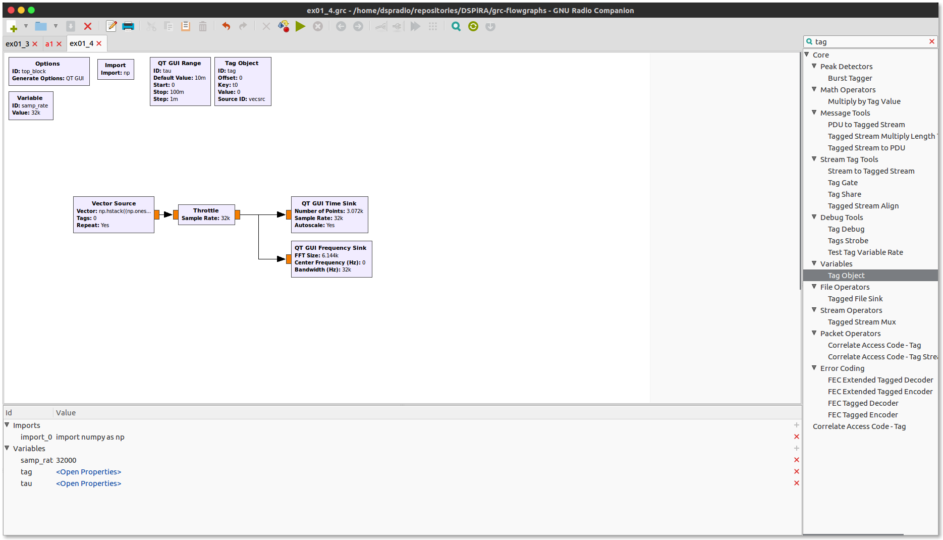
Use an “import” block to load a Python library. Use a “vector source” block to supply an arbitrary function. Start with a flowgraph like ex01_3.grc. Replace “signal source” with “vector source” and add an “import block”. Ignore the GUI elements for this exercise. We should have a flowgraph that looks like this:
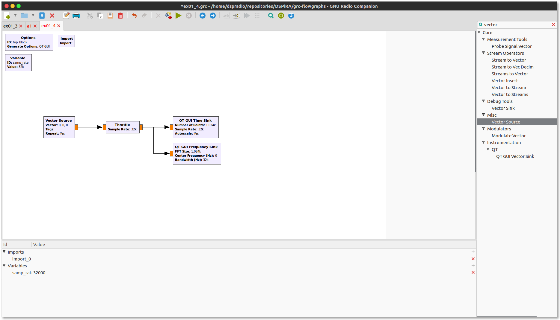
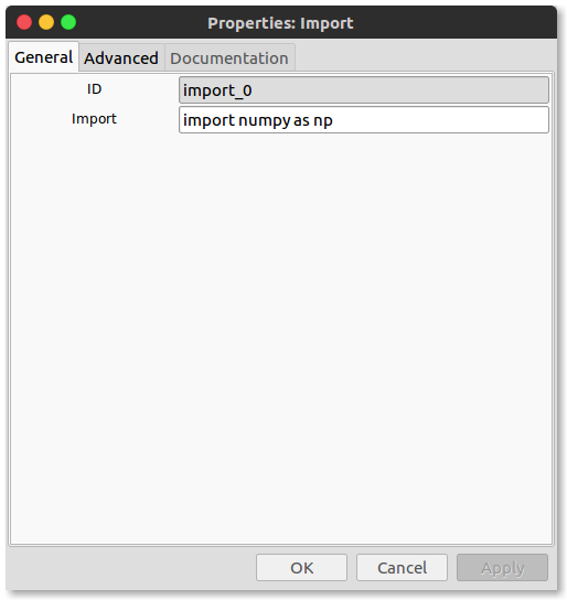
We shall import a standard library called numpy. It allows us to make matrices/vector and manipulate them easily. Double click the import block and fill out the import field as below:
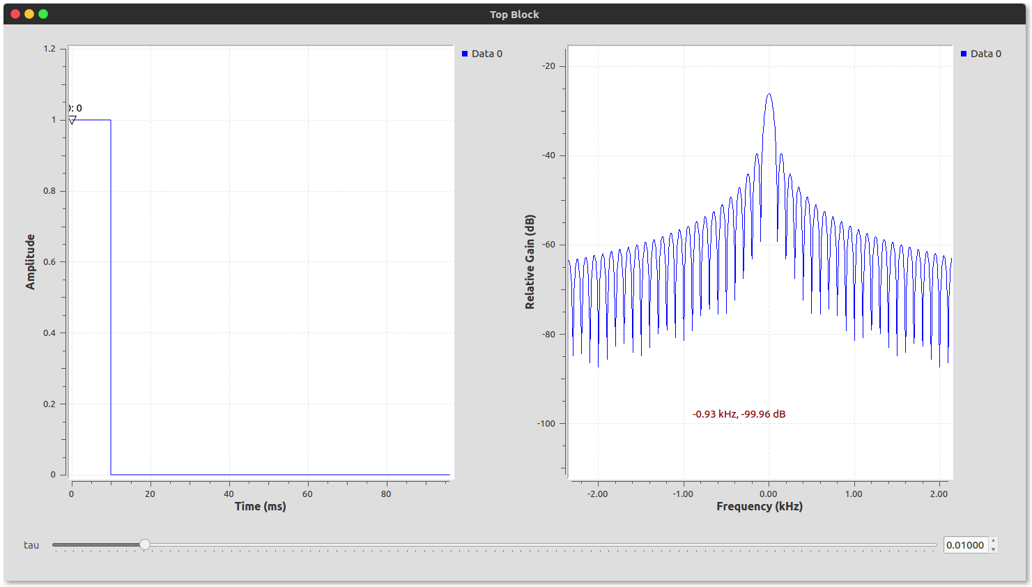
Create a rectangular pulse with adjustable width tau from 0 to 10 ms. Set that range using the “QT GUI Range block”
The function shall be generated shall be generated using the following python code:
np.hstack((np.ones(int(tau*samp_rate)), np.zeros(int((1-tau)*samp_rate))))
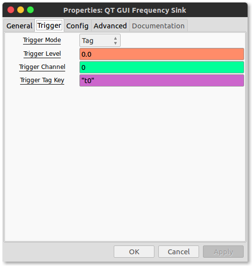
Before placing the blocks, consider a “Tag Object” block 1. It helps synchronize the sinks using a stream tag from the vector source. This lets us observe the generated pulse. Set the Vector Source “Repeat” field to “Yes” to repeat the pulse of width tau. Note the “Tag” field in the block properties shown below.
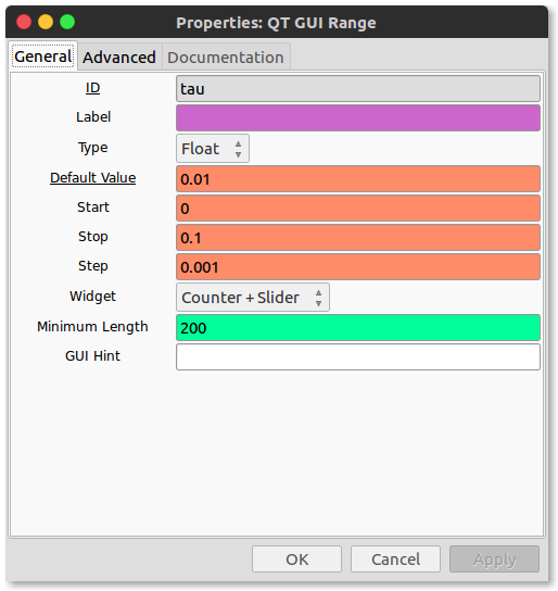
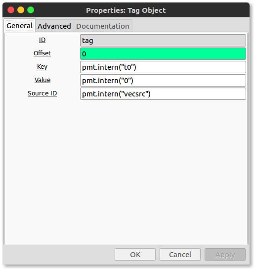
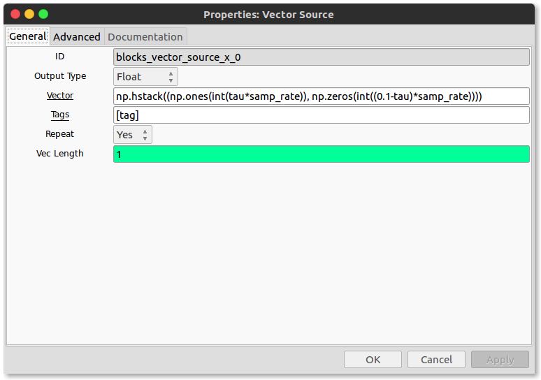
Set each sink’s trigger mode to “tag” and its “Tag Key” to t0. Set the time sink’s “Number of Points” to “samp_rate”. For the frequency sink, use “1024 * 6”. This is to properly visualize the signal and its frequency components.
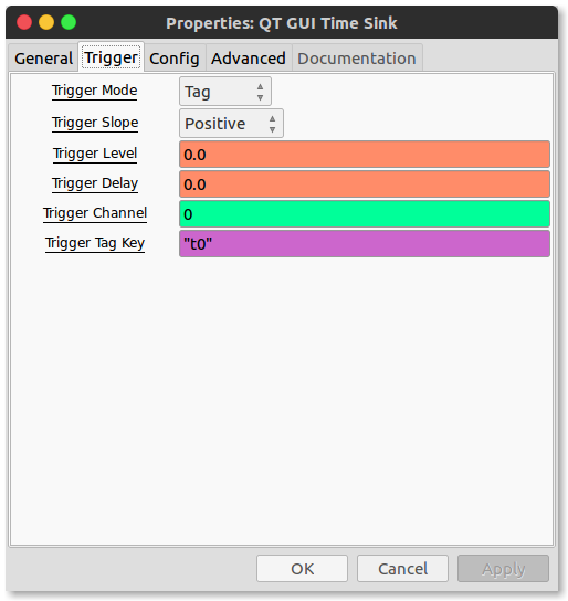
We should then have the flowgraph and output that looks like this:
1.5. Note on the Frequency Display
This particular display may not seem very intuitive for the those seeing it for the first time. It basically shows, as the name suggests, the ‘frequency’ components of the signal. This means the peaks in the graph represents the frequencies of the periodic signals that make up that particular signal. This is the basis of a very important concept called Fourier Analysis. Detailed discussions shall be done in class and systematically demonstrated in Lab 3 and Lab 5
1.6. Exercises
-
Delaying Signals: Add a “delay” block after the signal source. Control it with a “GUI Range” slider spanning 0 to 2000. See how the the signal changes in a time sink. NOTE: The delay value indicates the delay in units of number of time samples. Each time sample is \(\frac{1}{\verb+samp_rate+} \rm{s}\)
-
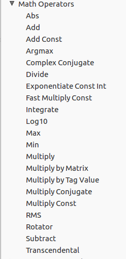
GNU Radio has a host of “Math Operators” that will allow you to perform a host of operations:
 .
.
Use multiple signal generators from section 1.3.3 to add and subtract and multiply to form new waveforms. We’ll add the examples here!
1.7. Random Discrete Signals
Think of a random signal as drawing numbered chips from a hat. An equation describes the relative abundance of each value: the ‘distribution’. One of the simplest is a uniform random signal, where each value has an equal number of chips.
In GNU Radio we can create these signals with a ‘Random Uniform Source’ block.
A very common distribution in nature is the ‘gaussian’ distribution.
1.8. Sampling
Sampling resembles drawing chips from the hat. Quantization rounds each chip’s value to the nearest integer. An analog-to-digital converter (ADC) measures a signal every clock cycle. It records the nearest available digital value.
1.9. Histograms
A histogram counts signal values within chosen intervals. Plotting the histogram is a way of trying to measure the distribution of an incoming random signal.
1.10. GNU Radio Companion Example.
Create the shown GNU Radio flowgraph.
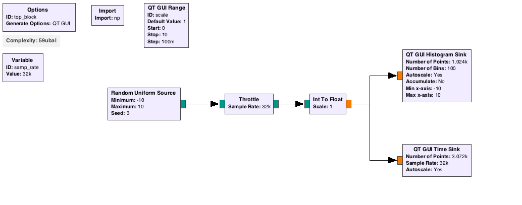
Use a random source between -10 and 10. The random source produces discrete integers. Add an Int to Float block with a ‘scale’ value to multiply each incoming sample.
Run the flowgraph, with the scale factor at 1. What does the time plot look like? What does the histogram look like? Now play with the scale factor. Can the histogram have large gaps? Can you make the histogram look continuous? What intuition do you gain from this about sampling a ‘random’ signal?
Now also try different distribution sources. Use the “Noise Source” block and set it to a gaussian distribution. What does the time stream look like? What about the histogram?
Now again use a cosine input signal as you’ve used in a previous exercise. What does the time series look like? The histogram? A cosine signal is not very random. What if each cosine sample occurred at a random time (equivalently, passing a uniform random signal through a cosine function)? Would the histogram look any different? The resulting signal is random, with the form \(\frac{A}{\sqrt{1-y^2}}\). It should agree with your histogram.
1.11. Make your own gaussian noise block
You are now ready to try to make your own gaussian noise block out of other blocks.
Create a new flowgraph in grc. We’ll start by using a just a QLFSR block. This is a ‘linear feedback shift register’ block, which is a very simple way to create ‘pseudorandom’ noise. Read about linear-feedback shift registers for more details. Set the type to float, the degree (how many elements in the shift register) to 32, repeat yes. Change the seed to any number. Leave the ‘mask’ at zero to get an ‘optimal’ source that wont repeat. Try using other numbers to compare, 1075838979 is a nice choice for random looking data. Use a histogram sink and a gui sink to look at the output. The output is only -1 or 1. It remains unpredictable without the initial seed and elapsed cycle count.
Add a number of these sources together:
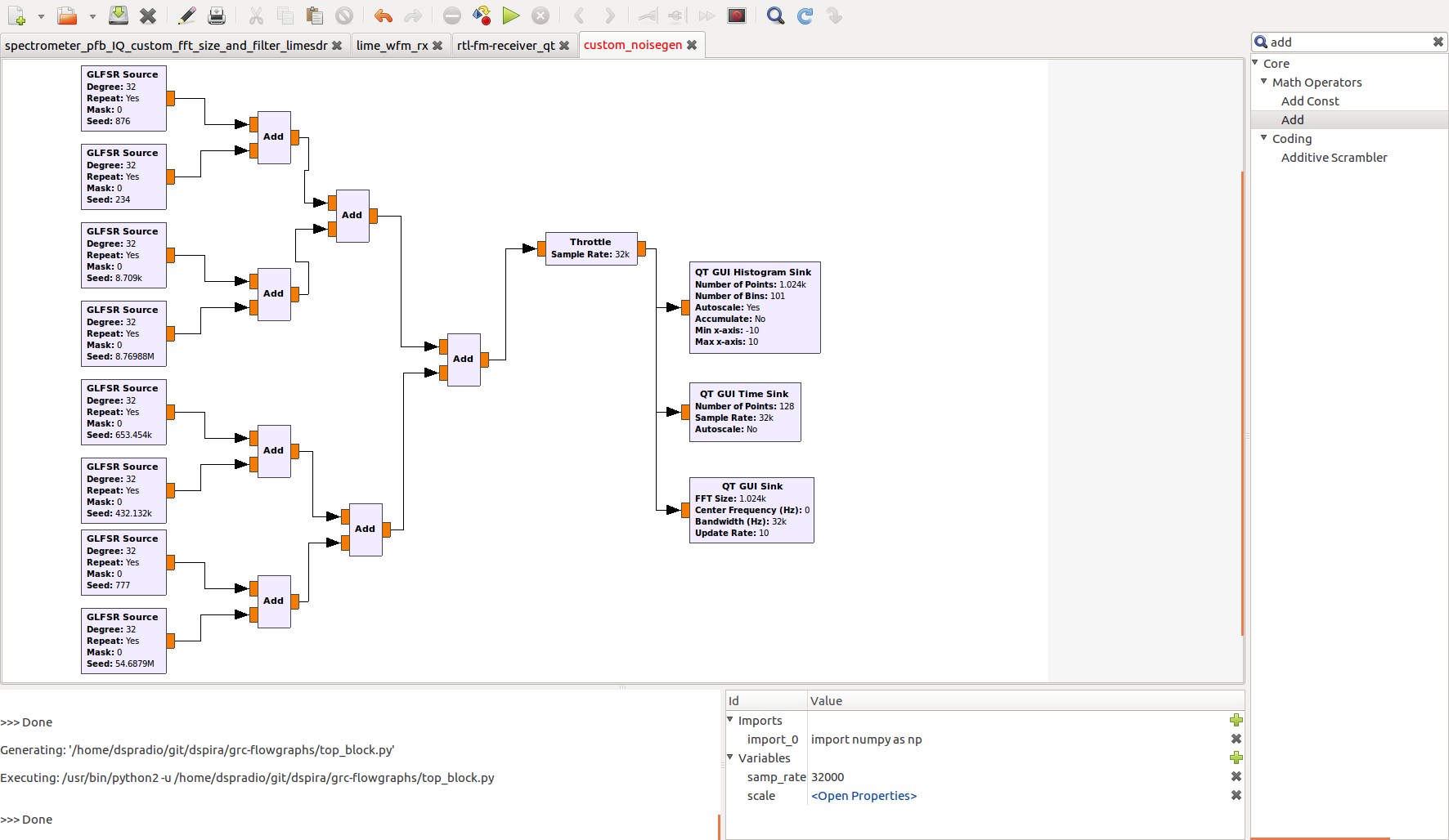
What does the output look like now? This is one of the simple ways of going from a ‘flat’ random number to a gaussian white noise.
↑ Go to the Top of the Page ……Next Lab
Extra Materials:
- A guided tutorial by GNU Radio
- This tutorial was adapted from Peter Mathys’s ECEN 4652 Communication Laboratory at the University of Colorado Boulder. The original lab website is no longer available.
-
For a technical explanation of the block click here Return to footnote 1 in the text