Every measurement a radio telescope makes is a correlation of some kind. A single horn correlates a signal with itself; two horns correlate one against the other. This lesson works through the three operations that underlie both — convolution, autocorrelation and cross-correlation — and then uses them to explain what a two-element interferometer actually measures.
It was written by Pranav Sanghavi at this lab in 2018. Everything here can
be run yourself: the notebook is at
code/interferometry/
and needs nothing but numpy, scipy and matplotlib.
- Convolution
- Cross-correlation and autocorrelation
- Why interferometry
- The two-element interferometer
- The effect of bandwidth
- Where to go next
- Credits
Convolution
\[(f * g)(x) \,=\, \int_{-\infty}^{+\infty} f(x-t)\,g(t)\,dt\]“In mathematics (and, in particular, functional analysis) convolution is a mathematical operation on two functions (f and g) to produce a third function, that is typically viewed as a modified version of one of the original functions, giving the integral of the pointwise multiplication of the two functions as a function of the amount that one of the original functions is translated”
for multiple dimensions
\[\begin{align} (f * g)(x_1,\ldots,x_n ) \,&=\, (f * g)({\bf x})\\ \,&=\, \int_{-\infty}^{+\infty} \ldots \int_{-\infty}^{+\infty} f(x_1-t_1, \ldots , x_n-t_n)\,g(t_1, \ldots, t_n) \,d^nt\\ \,&=\, \int_{-\infty}^{+\infty} f({\bf x}-{\bf t})\,g({\bf t}) \,d^nt\end{align}\]Properties of convolution
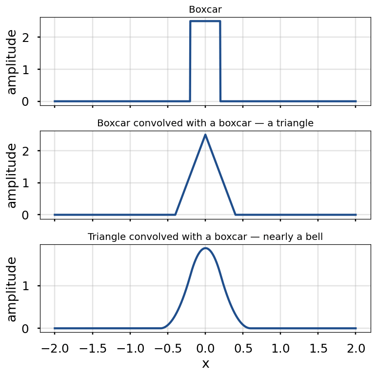
\[\begin{align} f * g \,&=\, g * f&\qquad (\text{commutativity})\\ (f * g)* h \,&=\, f * (g * h)&\qquad (\text{associativity})\\ f * (g + h) \,&=\, (f * g) + (f * h) &\qquad (\text{distributivity})\\ (a\, g) * h \,&=\, a \, (g * h)&\qquad (\text{associativity with scalar multiplication})\\ \end{align}\]Convolution smooths. Convolve a rectangle with itself and you get a triangle; convolve that with the rectangle again and you are most of the way to a Gaussian. That is the central limit theorem happening in front of you — repeated convolution drives almost anything towards a bell curve.
The reason this matters for a telescope is the next picture. Point sources on the sky are spikes. Your telescope has a beam — a response pattern roughly 15° across for a DSPIRA horn. What you record is the sky convolved with the beam.
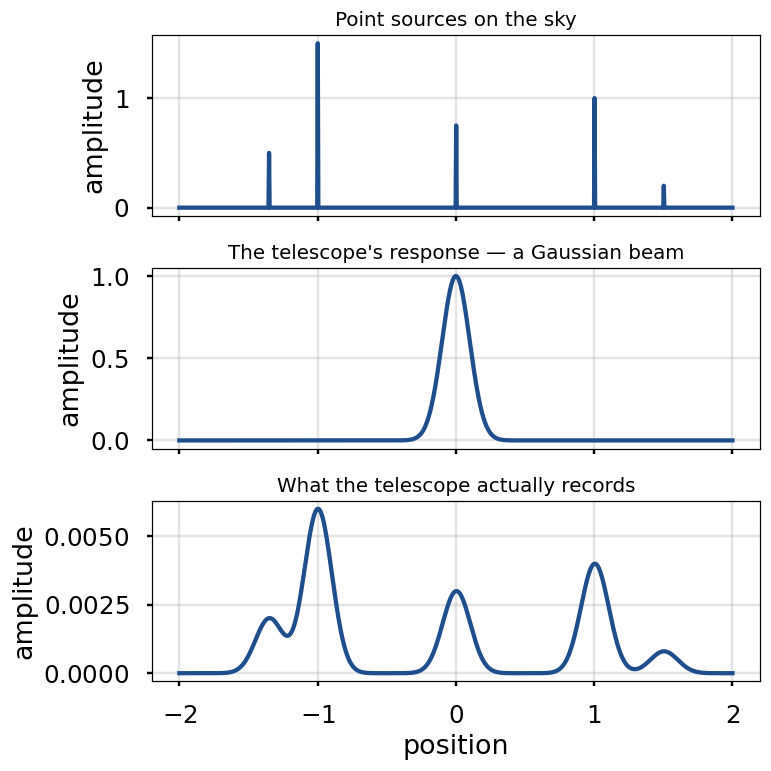
Two sources closer together than the beam merge into one bump. No amount of integration time separates them; the information is gone at the moment of measurement. That single fact is the whole motivation for interferometry.
Cross-correlation and autocorrelation
Cross-correlation asks how much two signals resemble each other when one is slid past the other:
\[\begin{split} (f\star g)(x) \,&=\, ({f_-}^*\circ g)(x)\\ &=\, \int_{-\infty}^{+\infty} f^*(t-x)\,g(t)\,dt\\ &\underset{t^\prime = t-x}{=}\, \int_{-\infty}^{+\infty} f^*(t^\prime)\,g(t^\prime+x)\,dt^\prime\\ \end{split}\qquad \text{,}\] \[\begin{align} (f\star g)(x_1,\ldots,x_n ) \,&=\, (f\star g)({\bf x})\\ &=\, ({f_-}^*\circ g)(x)\\ &=\, \int_{-\infty}^{+\infty} \ldots \int_{-\infty}^{+\infty} f^*(t_1-x_1, \ldots , t_n-x_n)\,g(t_1, \ldots, t_n) \,d^nt\\ \end{align}\]Autocorrelation is the same operation with one signal played against itself:
\[\begin{split} R\{f\}(x) \,&=\, (f\star f)(x)\\ &=\, (f_-^* * f)(x)\\ &=\, \int_{-\infty}^{+\infty} f^*(t-x)\,f(t)\,dt\\ &\underset{t^\prime = t-x}{=}\, \int_{-\infty}^{+\infty} f^*(t^\prime)\,f(t^\prime+x)\,dt^\prime\\ \end{split}\qquad \text{.}\]Note the difference from convolution: cross-correlation does not flip one of the functions, which is why \( f \star g \neq g \star f \) while \( f * g = g * f \).
Autocorrelation is how a radio telescope finds signal underneath noise. Below is a sine wave three times smaller than the noise it sits in — invisible in the raw trace. Its autocorrelation still shows the period, because the noise is uncorrelated with itself at any non-zero lag and the sine wave is not.
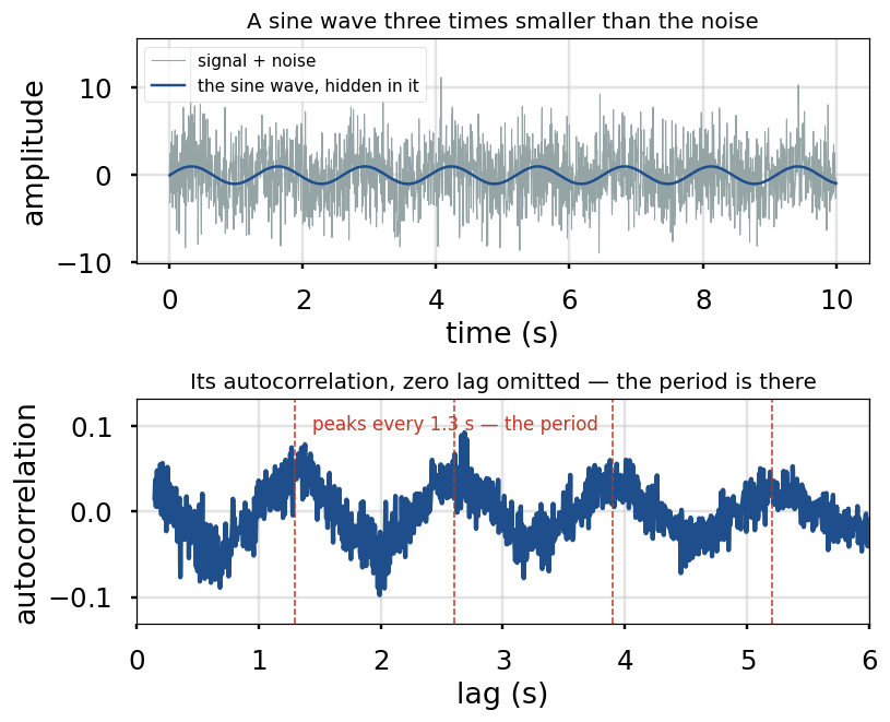
This is not an analogy for what the spectrometer does — it is what the
spectrometer does. The power spectrum you watch in
spectrometer_w_cal.grc
is the Fourier transform of the autocorrelation of the voltage coming out of
the horn. That equivalence is the Wiener–Khinchin theorem, and it is why the
hydrogen line rises out of a noise floor far larger than itself.
Why interferometry
The resolution of a single dish is set by diffraction:
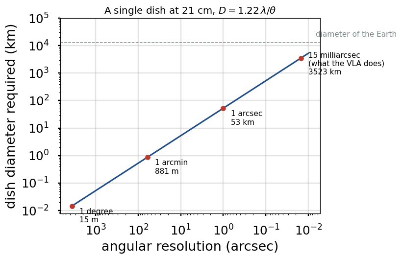
\[\theta \,\approx\, 1.22 \frac{\lambda}{D}\]At 21 cm that is a brutal constraint. Rearranged for the diameter you would need:
| You want | At 21 cm you need a dish |
|---|---|
| 1 degree | 15 m |
| 1 arcminute | 881 m |
| 1 arcsecond | 53 km |
| 15 milliarcseconds | 3,523 km |
The last row is the resolution the VLA reaches routinely. A single dish that did the same would be a quarter of the diameter of the Earth. You cannot build it, and this is not a matter of budget — it is a matter of the planet not being large enough.
The way out is to stop trying to fill the aperture and instead sample it at a few points. Two horns a distance \( b \) apart resolve detail on the scale \( \lambda / b \), with none of the collecting area of a dish that size, but all of the resolution.
The two-element interferometer
Take two antennas and combine their signals. There are two ways to do it:
- by addition, to form a sum interferometer, or \( \sum \)-interferometer
- by multiplication, to form a product interferometer, or \( \prod \)-interferometer
The sum interferometer
\[P ={2 V_0^2(1+ \cos\Delta \Phi)}\]The product interferometer
\[R_c= \langle V_1 V_2 \rangle_t\] \[R_c =\frac{V_0^2}{2}\cos{\omega \tau}=\frac{V_0^2}{2}\cos \Delta \Phi\]where \( \tau \) is the time delay in the signal path. The delay is geometric: a source at angle \( \theta \) from the zenith reaches one antenna before the other, by \( \tau = b\cos\theta / c \). As the Earth turns, that delay sweeps, and the output oscillates — the fringe.
This is a cosine correlator. Introduce an artificial phase delay of \( \pi/2 \) in one of the two signal paths and you get a sine correlator:
\[V_1=V_{01} \cos (\omega (t + \tau)) \quad V_2 = V_{02} \cos (\omega t + \frac{\pi}{2} )\] \[\begin{align} R&=\langle V_{01} V_{02} \cos{(\omega t + \frac{\pi}{2})} \cos{[\omega (t + \tau) ]} \rangle_t\\ R&= V_0^2 \frac{\langle \cos(2 \omega t + \tau + \frac{\pi}{2})+\cos (\omega \tau - \frac{\pi}{2})\rangle_t}{2} \end{align}\] \[R_s =\frac{V_0^2}{2}\sin{\omega \tau}\]Run both at once and you have a complex correlator, whose output is the visibility:
\[R = \int_{\Omega} I_\nu(\mathbf{s}) e^{-\imath 2\pi \frac{\mathbf{b}\cdot\mathbf{s}}{\lambda}} d\Omega = V\]That integral is a Fourier transform of the sky brightness. An interferometer measures the Fourier transform of the sky, one spatial frequency per baseline. Everything in aperture synthesis follows from it.
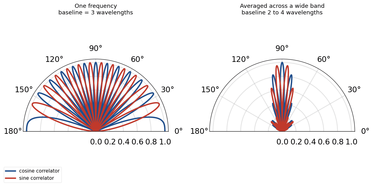
Here is the fringe pattern of a two-element interferometer with a baseline three wavelengths long — the left panel. The lobes are the directions where the two paths arrive in phase.
The effect of bandwidth
The right panel above is the same interferometer observing across a wide band rather than at one frequency. The baseline measured in wavelengths changes across the band, so each frequency puts its lobes in a slightly different place, and averaging them washes the pattern out — except near \( \theta = 90^\circ \), where the geometric delay is zero and every frequency agrees.
This is bandwidth decorrelation, and it has a practical consequence: a broadband interferometer only sees clearly near the direction where its delays are matched. Real arrays fix this by inserting a compensating delay that tracks the source, so the zero-delay direction follows what you are looking at instead of sitting at the zenith.
For the DSPIRA two-horn setup, the equivalent lesson is that the fringes are sharpest for sources transiting near the phase centre, and that narrowing the band widens the region over which fringes survive — at the cost of sensitivity.
Where to go next
Two elements give you one spatial frequency at a time. Rotating the Earth sweeps that baseline through the Fourier plane, and adding antennas fills it in faster — that is aperture synthesis, and it is where this subject really opens up.
The standard treatment is Fundamentals of Radio Interferometry, the course book from Rhodes University and the National Astrophysics and Space Science Programme. It is free to read, it is written as runnable notebooks like this one, and chapter 4, Visibility Space, picks up exactly where this page stops. Start there.
Closer to home, and worth doing in this order:
- Additive Interferometry Using Two DSPIRA Radio Horn Telescopes — LightWork Memo 31. The same fringe pattern as above, but measured: a transit of the sun on a 5.0 m baseline, fringe spacing 0.043 rad against 0.042 rad predicted. This is what the theory on this page looks like when it comes out of a real horn.
- Setting up a 2 Horn Interferometer — building one and running it
- Interferometry — the rest of the interferometry material on this site
- Fourier Analysis and Expert Mode — the transforms this page leans on
Credits
The text, equations and code on this page were written by Pranav Sanghavi at the WVU Radio Astronomy Instrumentation Laboratory on 21 May 2018, and are published here under this site’s MIT licence. The notebook was ported from Python 2 to Python 3 in 2026; the autocorrelation figure was added then, and everything else is his.
The definition of convolution is quoted from Wikipedia under CC BY-SA 4.0.
Fundamentals of Radio Interferometry is a separate work by the Rhodes University Centre for Radio Astronomy Techniques & Technologies and the NASSP community, licensed GPL v2. It is linked above rather than reproduced.