Observations - Mapping the Sky and Measuring the Rotation Curve

Let’s use our telescopes.

Use this lab once the spectrometer works. It shows how to extract scientific results from saved observations. It was DSPIRA’s Lab 7, written for the summer workshop, and it is the command-line route through the data.

Looking for the classroom version? The Velocity Curve of the Milky Way lesson covers the same measurement. It uses student handouts and a spreadsheet instead of Python. Same physics, different audience. Read that one if you are teaching this to a class; read this one if you want the pipeline.

The scripts are in code/observations/. The README explains installation and each script’s output.

1. Reading the data with Python

Install Python and Jupyter:

sudo apt install ipython3 jupyter

What you do next depends on which sink you used.

If you used the plain file sink

The data is float32 in 4096-point vectors, packed end to end with nothing to say so. Open IPython in the folder where the data is:

ipython3 --pylab

##########################
## Read and reshape data
##########################

spec = np.fromfile("data", dtype=np.float32)  # read the whole file as one long array
spec.shape                                    # how many numbers is that?
spec = spec.reshape((-1, 4096))               # stack it into 4096-point spectra
spec.shape                                    # first number is now the count of integrations

###############################################
# save to a text file to open in a spreadsheet
###############################################

np.savetxt("reshapeddata.csv", np.transpose(spec), delimiter=',')

##############################################
# Plot
##############################################

plot(spec[0])   # the first integration
plot(spec[i])   # the i-th integration

If you used the hdf5_sink out-of-tree module

The file carries its own metadata, which is why this is the better choice.

##########################################
# Import h5py to read hdf5 files
##########################################

import h5py

###########################################
# read the file into a variable
###########################################

f = h5py.File('2017-07-19_16.12.50.h5', 'r')

list(f.attrs)          # what metadata is there
list(f.attrs.items())  # metadata and values
f.items()              # what datasets are in the file

#############################################
# extract the spectrum data
#############################################

spectrum = f['spectrum'][:]

###############################################
# save to a text file to open in a spreadsheet
###############################################

np.savetxt("reshapeddata.csv", np.transpose(spectrum), delimiter=',')

############################################
# plot it against real frequency
############################################

fstart = f.attrs['freq_start']    # first channel, in Hz
fstep = f.attrs['freq_step']      # channel width, in Hz
flength = 4096                    # number of channels
freq = np.arange(flength)*fstep + fstart
rcParams['axes.formatter.useoffset'] = False
plot(freq, 10.0*np.log10(spectrum.mean(axis=0)))   # take the log here, for a dB display

hdf5_to_csv.py does that conversion for you if you would rather not type it.

2. A drift map of the sky

Calibrate first. Point at the ground for the hot load. Use an empty patch of sky for the cold load. That lets you put the data in units of temperature, which is what makes separate observations combinable.

python3 convert_to_temperature.py -g gnd.h5 -s sky.h5 -o tsys.pdf

Then observe. Point the telescope at a fixed spot and record for as long as possible. South along the meridian works well. That is drift scanning: you hold still and let the sky turn past you.

After 24 hours you have a full circle of sky at that elevation. Move up by 10 degrees, about half a beam width, and go again. A few weeks of that maps the whole sky.

Write down the pointing. Not in a notebook — in the file. The pointing box in the hdf5_sink block is the only record of the telescope’s aim. The map script needs this information. Write azimuth then elevation in degrees, like A180E40, before you start recording.

The block ships with AZ,EL in that box. That is a placeholder. A file saved with it cannot be mapped.

Everything else you can think of — your location, the telescope, the weather — goes in the notes box. You will not remember anything you did not write down.

Turning the observations into a map

python3 map_h1_hdf5_drift.py -d ~/my_observation/ -n -79.872 -l 39.659 \
        -s airspy -g tsys_gain.csv -t tsys_Tsys.csv

-n is your longitude, negative if west. -l is your latitude. Both default to Green Bank. -s selects your radio: airspy, airspy-mini, pluto, lime or rtlsdr. Their recorded bandwidths differ, so this setting determines the script’s frequency windows. An incorrect setting produces an error instead of an empty map. -g and -t specify the previous step’s calibration files. Without them, the map uses raw units instead of temperature.

If you use an RTL-SDR, check freq in the flowgraph before you observe. It has to be 1420.5e6, not the default 1419e6. At a 2.4 MHz sample rate, the default records 1417.8 to 1420.2 MHz. The hydrogen line at 1420.4058 MHz lies outside that band. The telescope works but records no hydrogen. The source block settings page has the full list per radio.

python3 map_h1_hdf5_drift.py --help lists everything.

That writes two files into the directory you are standing in:

The map is h1map / hitmap — signal divided by exposure. Open both in a spreadsheet and divide one by the other, or let Python do it:

mkdir ~/my_observation_map
cp h1map_drift.csv hitmap_drift.csv ~/my_observation_map/
python3 map_from_csv.py -d ~/my_observation_map/

That draws the map in galactic coordinates and saves gal_map.pdf. Put several observations’ csv files in the same directory — give them distinct names — and they are combined into one map.

A warning about dividing by zero is expected. Pixels you have not looked at yet have no hits, so they come out blank. A partial map is supposed to have holes.

3. The rotation curve of the Milky Way

Use Stellarium or similar to plan. Stay in quadrant I — galactic longitude between 0° and 90°. The tangent point method requires a line of sight inside the Sun’s orbit. This means \(|l| < 90°\). (Quadrants II and III reveal galactic rotation, as shown in Part 1 of the classroom lesson. Their lines of sight have no tangent point. They cannot yield a rotation curve with this method.)

Point along the galactic equator, step by 10 degrees, and record 30 seconds to 5 minutes at each pointing. Record the pointing in the file, as above.

From frequency to velocity

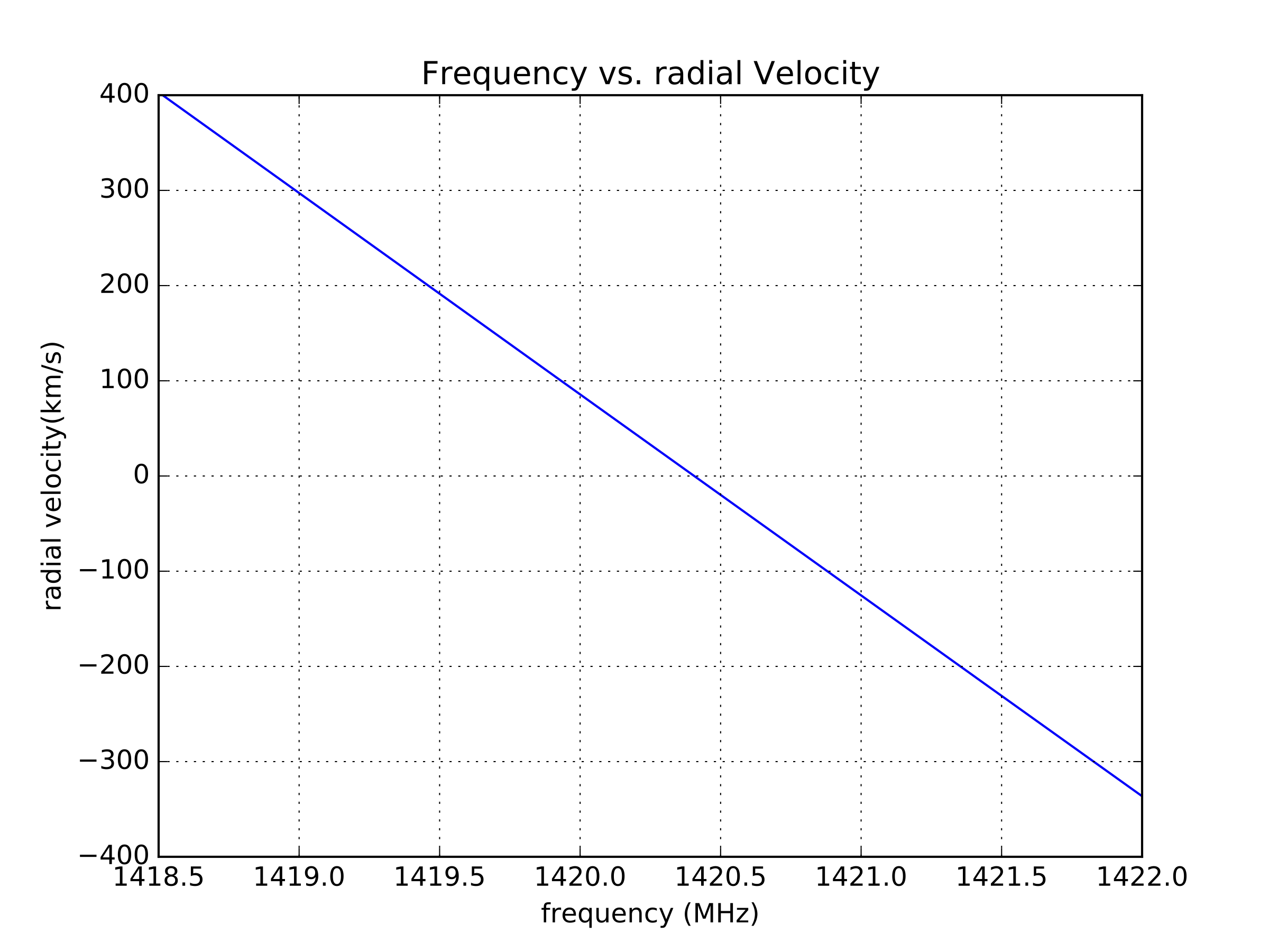
Neutral hydrogen emits at 1420.40575177 MHz. We see it at other frequencies because it is moving relative to us. Non-relativistically:

where \(\lambda_e\) is the wavelength emitted and \(\lambda_o\) the wavelength observed. Using \(c = \lambda f\) to get to frequency:

with \(f_e\) the frequency emitted, \(f_o\) the frequency observed, and \(c\) = 300,000 km/s.

You can now turn power against frequency into power against speed relative to us. Does it matter what units the frequency is in?

From velocity relative to us, to velocity around the galaxy

What we want is how fast hydrogen orbits the galactic centre, as a function of how far out it is. What we measure is its speed along one line of sight.

Use 200 km/s for the Sun’s orbital speed; estimates range from 180 to 250 km/s. Use an orbital radius of 8 kpc, with roughly 1 kpc uncertainty. (The Earth’s 30 km/s around the Sun matters for a careful measurement. Skip it for now.)

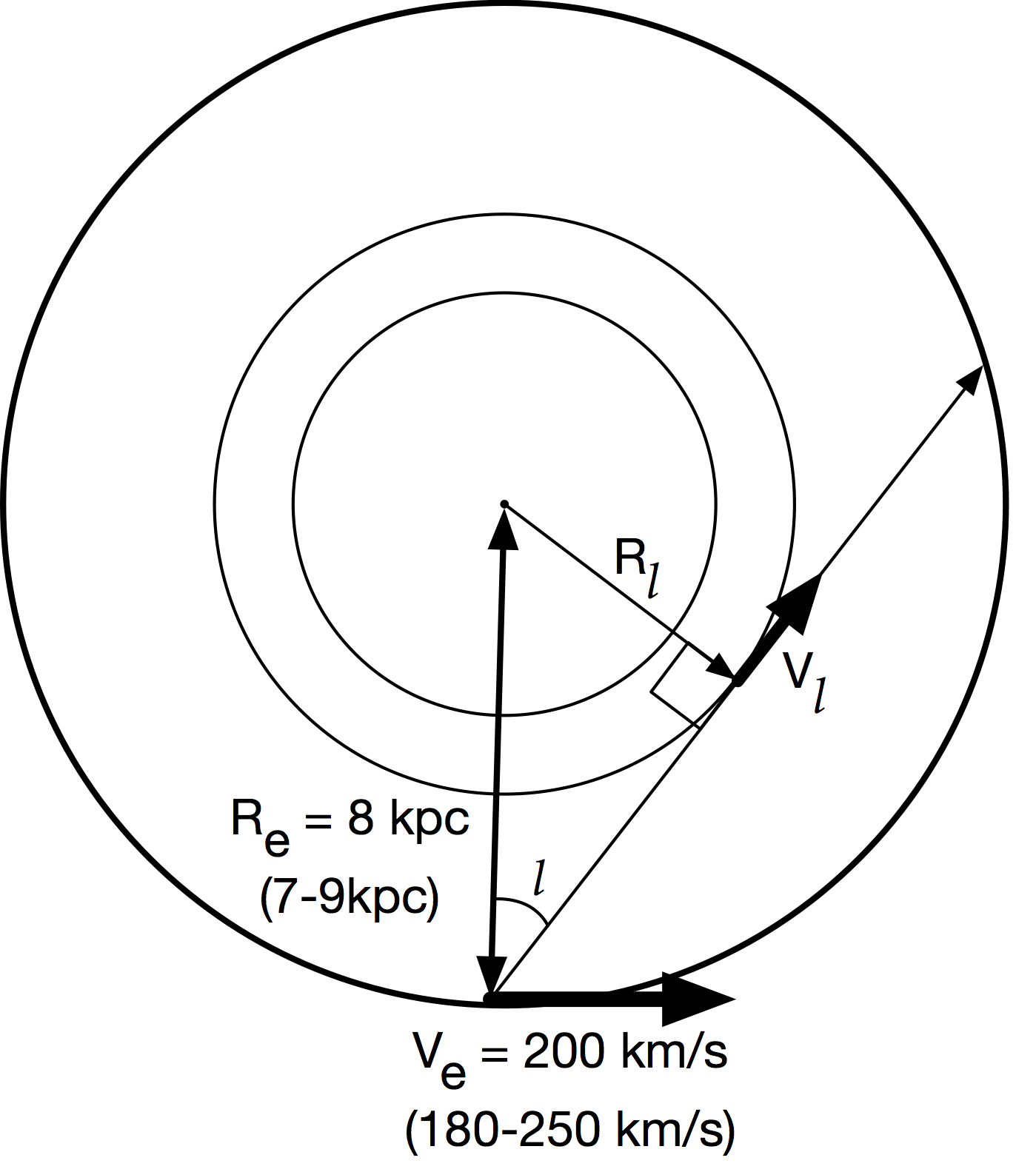
Use the tangent point method. Assume the fastest hydrogen along a sightline lies closest to the galactic center. Its orbital motion follows your line of sight there. So take the most extreme velocity you measured — most negative or most positive — at each galactic longitude.

The radius that corresponds to is

with \(R_e\) the Sun’s distance from the centre and \(l\) the galactic longitude — valid, again, only for \(|l| < 90°\). The rotation speed there is

with \(V_{los}\) the extreme velocity at that longitude and \(V_e\) the Sun’s orbital speed.

Plot \(V_l\) against \(R_l\) and you have a rotation curve for the Milky Way.

What did you expect it to look like? Compare it against what a galaxy with all its mass in the visible disc would give you.

A worked example: the Green Bank Telescope

The 2017 DSPIRA cohort connected their new spectrometer to the Green Bank Telescope. They recorded a 24-hour drift scan. That notebook is here, with the calibration worked through:

• GBT drift scan notebook

The data file remains on Green Bank’s systems and is not included. This notebook reverses that observation’s intermediate-frequency downconversion and corrects a clock error. It also selects integration ranges specific to that file. Read it as a worked example. Before applying it to your data, follow the README’s instructions for adapting it. Comparing a horn telescope’s spectrum against a 100 m dish’s is worth the detour.

Where this lab stops

The original lab had three empty sections: beam pattern measurement, horn improvements, and combining multiple horns. They were never written.

Two of the three are covered elsewhere on this site:

• Combining horns: Setting up a 2 Horn Interferometer and Interferometry
• Horn variations: Other Horn Designs

Beam pattern measurement is genuinely missing. If you have measured one, that would be a good thing to contribute.